Feature Engineering for ML (Part 13): Trend-Scanning Features in Python

Table of Contents

1. Introduction
2. What Trend-Scanning Measures
3. One Function, Two Calling Conventions
4. The Wrapper: Isolating the Causal Feature Slice
5. Verifying the Backward Window Is Actually Backward
6. Two Defects Found While Building the Wrapper
7. Results: Quantifying Both Defects
8. Feature Output on Realistic Data
9. The Selection Rule Does Not Select Significance
10. Conclusion
11. References
12. Attached Files

Introduction

The MetaTrader 5 Machine Learning Blueprint series introduced trend-scanning as a labeling method: fit OLS regressions over several candidate window lengths, keep the window with the largest absolute t-value, and use its sign as the label. That function, trend_scanning_labels, lives in afml.labeling.trend_scanning and has not changed since. What changes in this article is the question asked of it. A label answers "what happened after this bar." A feature must answer "what was knowable at this bar," and the same function can be made to answer either question, because it exposes both directions through a single argument.

This is a different failure mode than the ones covered so far in this series. Part 11 found a leak baked into a centered rolling window with no causal option available at all, and Part 12 carried the corrected, causal fractal features across to their MQL5 port. Here the causal option already exists: lookforward=False is a first-class, tested code path. The risk is using the labeling-appropriate default when building a feature matrix. Nothing in the function signature prevents the call from succeeding. It returns a well-formed DataFrame that looks correct.

This article wraps trend_scanning_labels in a feature-only interface that removes the choice rather than documenting it. It measures the leak caused by the wrong choice and documents a second, unrelated defect that appears when the function is applied to a signed input series rather than raw price.

It also covers a third finding, separate from either of the defects above and concerned with the method rather than the code. The rule for choosing among candidate windows does not select the most significant trend, and the t-value it returns cannot be read against the nominal Student-t threshold on price data. Both claims are established by simulation.

What Trend-Scanning Measures

For a window of length L ending (or starting) at some bar, the function fits price against a time index by ordinary least squares and keeps three numbers: the slope, the R², and the t-value on the slope. It repeats this for every L in a candidate span and keeps the window whose |t-value| is largest. The sign of the t-value gives the direction. Its magnitude measures how confidently a straight line explains the window, while accounting for the number of points in the fit (Lopez de Prado, Lecture 3/10).

The result behaves differently from a fixed-window slope in one useful respect: the window length is chosen per bar rather than fixed for the whole series. A sharp two-bar move and a shallow twelve-bar drift can both register as a strong trend, at different L, without either being diluted by forcing one window length on both.

The Numba kernel that does the fitting, _window_stats_numba, computes all three statistics from the same set of running sums in one pass per window, which is what makes scanning a dozen or more candidate lengths across thousands of bars practical:

@njit(parallel=True, cache=True)
def _window_stats_numba(y, window_length):
    n = len(y)
    num_windows = n - window_length + 1
    t_values = np.empty(num_windows)
    slopes   = np.empty(num_windows)
    r_squared = np.empty(num_windows)

    t = np.arange(window_length)
    mean_t = t.mean()
    Var_t  = ((t - mean_t) ** 2).sum()

    for i in prange(num_windows):
        window = y[i : i + window_length]
        mean_y = window.mean()
        S_ty   = (window * t).sum()
        slope  = (S_ty - window_length * mean_t * mean_y) / Var_t
        # SSE, R², and the t-value follow from the same running sums
        ...

Two masking steps sit around this kernel and are worth naming before Section 3, because both survive unchanged in either calling direction. volatility_threshold zero-masks any window whose local standard deviation falls below an expanding quantile, so a flat, quiet stretch cannot register a spurious trend from rounding noise. And a window's t-value is only trusted if it clears both this volatility floor and, downstream, an absolute threshold of 1e-6 before it contributes a nonzero sign.

One Function, Two Calling Conventions

The direction of the fit is controlled entirely by lookforward. With it True, the default, the valid range excludes only the last max(span) bars and each window starts at the current bar and extends forward:

if lookforward:
    valid_indices = close.index[:-max_hrzn].to_list()
else:
    valid_indices = close.index[max_hrzn - 1 :].to_list()

The forward case is correct for labeling: the whole point of a label is to describe what happens after the event it is attached to. The backward case is what a feature needs: the window ends at the bar carrying the feature, so nothing in it was unknowable at that timestamp.

Making the backward case work from the same forward-only kernel is done by reversing the series, running the same windowed fit, and reversing the result back:

y_window = y if lookforward else y[::-1]
t_vals, slopes, r_sq = _window_stats_numba(y_window, hrzn)
if not lookforward:
    t_vals, slopes, r_sq = t_vals[::-1], slopes[::-1], r_sq[::-1]
    start_idx = hrzn - 1
else:
    start_idx = 0

This is the one place in the function where getting the index arithmetic wrong would be easy and silent: a reversed array that is placed back at the wrong offset would still produce a full column of plausible-looking numbers. checks it directly rather than taking the offset on faith.

Both directions return the same seven columns — t1, window, slope, t_value, rsquared, ret, bin — because the function was written for one purpose and the backward mode was added as an option on the same output shape. Three of those columns describe the outcome the window was chosen to explain, not a property available at the feature's own timestamp, and that distinction does not change when lookforward does.

The Wrapper: Isolating the Causal Feature Slice

The fix is not to change trend_scanning_labels, which is correct for its original purpose and used elsewhere in this series for exactly that. It is to give the feature use its own entry point that cannot be pointed the wrong way:

def get_trend_scanning_features(close, span=(5, 20), volatility_threshold=0.0,
                              use_log=True):
    """Causal trend-scanning features: window, slope, t_value, rsquared."""
    raw = trend_scanning_labels(
        close, span=span, volatility_threshold=volatility_threshold,
        lookforward=False, use_log=use_log,
    )
    return raw.drop(columns=["t1", "ret", "bin"])

There is no lookforward parameter on this function, and that omission is the point. A wrapper that accepted the argument and defaulted it to False would still let a caller pass True and rebuild the leak one keyword away. Removing the parameter removes the call that would do it.

The three dropped columns are not wrong, they are answers to the wrong question for a feature matrix. t1 and ret describe the endpoint and return of the chosen window, which for the causal direction is simply t itself and therefore redundant, but for the forward direction used in labeling is exactly the outcome being predicted. bin is the label. Feeding any of the three into X alongside a y built from the same function is the trend-scanning version of the min_ret role conflation documented in the transaction-cost article: two different jobs for the same underlying quantity, merged by sharing a variable name.

Verifying the Backward Window Is Actually Backward

Trusting a reversal-and-reindex trick without checking it is exactly the habit this series argues against. The claim to verify is that position t in the backward output holds the fit of close[t-L+1 : t+1], using nothing from t+1 onward.

The check is direct: run the function forward and backward on the same series, and confirm that the backward output at bar t equals the forward output at bar t-L+1 for the corresponding window length, since both describe the identical span of prices fit in the identical direction.

fwd = trend_scanning_labels(close, span=(5, 20), lookforward=True)
bwd = trend_scanning_labels(close, span=(5, 20), lookforward=False)

# bwd.loc[t] used window [t-L+1, t]; the forward call that fit the same
# span starts its window at t-L+1, so it is indexed there, not at t
L = bwd.loc[t, "window"]
match = fwd.loc[t - L + 1, ["slope", "t_value", "rsquared"]]
assert np.allclose(bwd.loc[t, ["slope", "t_value", "rsquared"]], match)

When run across a synthetic series, this held exactly for every bar where both a forward and a backward fit existed for the matching window length, at floating-point precision. The reversal is implemented correctly; the risk the rest of this article documents is entirely at the call site, not inside the kernel.

Two Defects Found While Building the Wrapper

6.1 Nothing in the API distinguishes the two use cases

The signature of trend_scanning_labels does not indicate that lookforward=True is unsafe for a feature matrix. The docstring calls the function a labeling technique, but the parameter list, the return shape, and the column names are identical in both directions, and a reader assembling a feature matrix by analogy with the fractal or entropy wrappers earlier in this series would have no reason to expect a fourth argument to matter this much. measures what calling it with the default produces.

6.2 use_log silently reinterprets a signed input

The function's own parameter is named close and its docstring assumes a raw, strictly positive price series. Nothing enforces that. A natural second use of trend-scanning inside this series is to run it over an already-engineered signed column — an FFD output, a return series — to ask whether that column itself is trending. With the default use_log=True, the function clips every value below 1e-8 to that floor before taking a log:

if use_log:
    close_processed = close.clip(lower=1e-8).astype(np.float64)
    y = np.log(close_processed).values

On a series that crosses zero, every negative value collapses to the same constant before the fit ever runs. This raises no exception, changes no output shape, and returns numbers that look like ordinary t-values.

Results: Quantifying Both Defects

Both defects were measured rather than asserted. The leak was tested on 3,000-bar synthetic random walks, twenty seeds, with no genuine trend anywhere in the data-generating process. For each bar, the sign of the trend-scanning t-value was compared against whether the next bar's close was higher or lower. On pure noise this comparison should sit at 50%; any persistent deviation is leakage, since there is nothing in the process to predict.

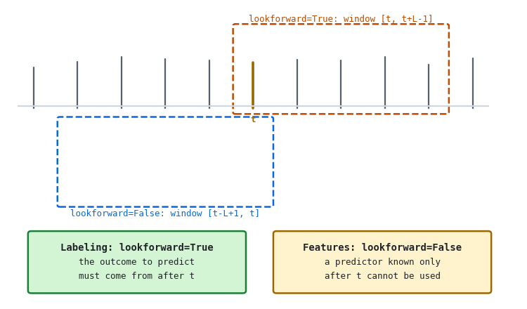
Figure 1. Single-panel illustration of the forward and backward windows produced by the same function

• Top: a candidate bar t, with the forward window [t, t+L-1] and backward window [t-L+1, t] both shown against it.
• Bottom: the forward window is the correct choice for labeling, because a label is allowed to describe the future. The backward window is the only correct choice for a feature.

Sweeping the maximum candidate horizon from 8 to 32 bars shows the leaky mode holding a hit rate between 56% and 61% across the range, against 49.9%-50.1% for the causal mode at every setting:

Max horizon	Leaky (lookforward=True)	Causal (lookforward=False)	Gap
8	0.6102	0.5004	0.1098
12	0.5912	0.4997	0.0915
16	0.5809	0.4992	0.0817
20	0.5746	0.5014	0.0732
26	0.5644	0.5013	0.0631
32	0.5584	0.4999	0.0585

The gap narrows as the horizon grows, rather than widening. That is the opposite direction from the centered-window leak in Part 11, and worth being precise about rather than forcing it to match that earlier pattern. This test only checks agreement with the single next bar. As the candidate span extends to longer horizons, the optimizer increasingly selects longer windows to maximize |t-value|, and a longer window's fit result correlates less tightly with any one specific bar inside it, including the next one. The leak does not shrink; the fraction of it visible to a one-bar-ahead test does.

The second defect was measured on a synthetic mean-reverting series standing in for an FFD or return column, where 44.7% of bars fall below the 1e-8 clip floor and collapse to the same constant before the log transform. Comparing the resulting t-values against a use_log=False fit on the identical series, computed causally in both cases, the sign disagrees on 18.3% of bars and the two t-value series correlate at 0.80 rather than 1.0.

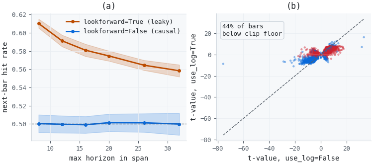
Figure 2. Two-panel illustration of both defects, measured rather than asserted

• Panel (a): next-bar hit rate on pure random-walk data across a sweep of the maximum candidate horizon, with one standard deviation shaded across twenty seeds.
• Panel (b): t-value under the default log transform against the linear fit on the same signed series, colored by whether the input bar fell below the clip floor.

Feature Output on Realistic Data

The wrapper's output on a 500-bar synthetic series with three injected drift regimes shows the optimal-window selection and R² behaving as intended: short, confident windows during the drift regimes, longer and noisier ones in between.

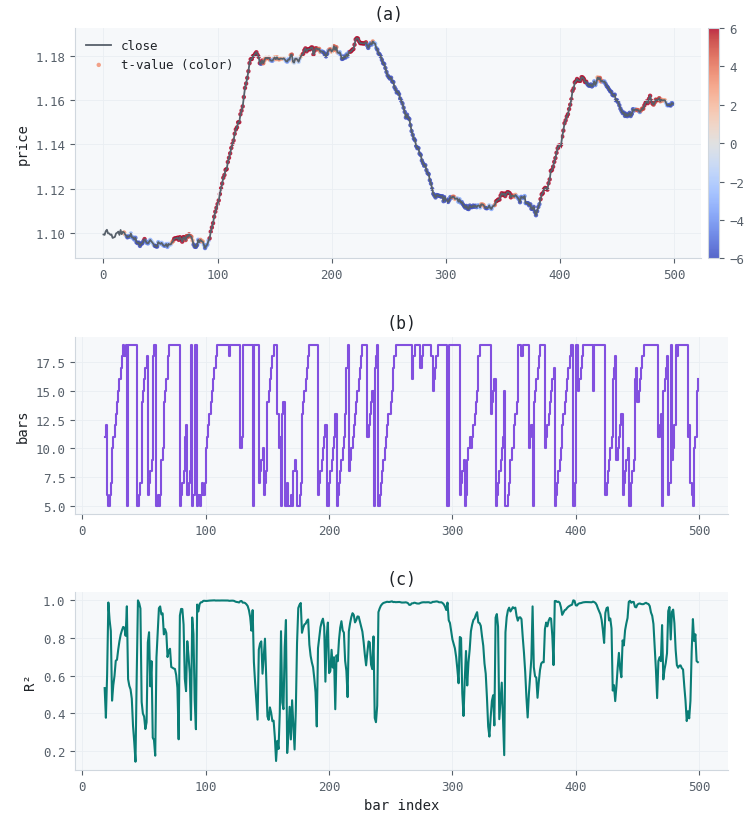
Figure 3. Three-panel illustration of the wrapper's output over 500 synthetic bars

• Panel (a): close price colored by the t-value at each bar, using only information available up to that bar.
• Panel (b): the window length selected by the argmax step, which steps as the data favors a shorter or longer fit.
• Panel (c): R² of the chosen window, higher during the three injected drift segments than in the surrounding noise.

This section clarifies what the results do and do not establish. The regimes were injected, so panels (b) and (c) confirm that the optimizer finds a cleaner fit where one was placed and nothing more. It says nothing about how these features would behave against real structure, which is a question for the modeling stage, not the feature stage.

The Selection Rule Does Not Select Significance

Everything so far treats trend_scanning_labels itself as correct, and confirmed that the backward mode is. This section is about something else: the rule the function uses to choose among the candidate windows it fits, which is correct as an implementation of Section 5.4 of Machine Learning for Asset Managers and does not do what that section says it does.

The rule is argmax|t|: fit every horizon in the span, keep the one whose absolute t-value is largest.

best_j = np.nanargmax(np.abs(t_block), axis=1)

A t-value is referred to a Student-t distribution with L - 2 degrees of freedom, and that distribution's shape depends on L. A five-bar window has three degrees of freedom and heavy tails; a forty-bar window has thirty-eight and is close to normal. The same numerical t-value therefore represents different amounts of evidence depending on which window produced it, and taking a maximum over raw t-values compares quantities measured on different scales. It systematically favors the shortest windows in the span.

A deterministic series shows how large the effect is. Take y[i] = 100 + 0.05i + 3sin(0.3i), fit it on log price, and evaluate every window from 5 to 40 bars ending at bar 199:

L= 5: t=-12.840  p=1.02e-03   # selected by argmax|t|
L=20: t= +6.572  p=3.57e-06   # 286x more significant, discarded

The rule selects the window that is roughly 286 times less significant. The two windows also disagree about direction: the five-bar fit is falling and the twenty-bar fit is rising, so the published rule reports a downtrend on a bar where the stronger evidence points up. This is not a constructed edge case — it happens whenever a short reversal sits inside a longer move, which on intraday data is common.

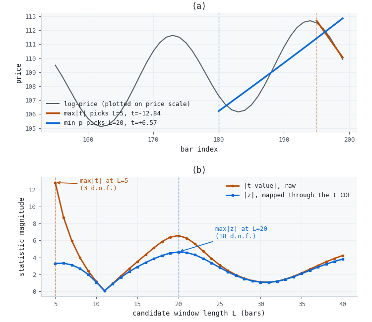
Figure 4. Two-panel illustration of the two selection rules reaching opposite conclusions on one bar

• Panel (a): the five-bar window chosen by the raw rule and the twenty-bar window chosen after length correction, both fitted on the same final bar and pointing in opposite directions.
• Panel (b): the profile of both statistics across the candidate span, showing raw absolute t-value peaking at the short end while the corrected statistic peaks near twenty bars.

The correction is one line longer than the rule it replaces. Converting each candidate to a p-value before comparing removes the dependence on window length, because a p-value is already expressed on a common scale:

from scipy import stats

# t_block has shape (n_events, n_horizons); each column carries its own
# degrees of freedom, so the survival function is evaluated per column.
df = np.asarray(hrzns) - 2
p_block = 2.0 * stats.t.sf(np.abs(t_block), df[None, :])
best_j = np.nanargmin(p_block, axis=1)

The wrapper exposes this as a selection argument rather than switching the default, so pipelines already built on it keep the behavior they were validated against. selection="max_abs_t" reproduces the published rule exactly; selection="min_p" applies the correction. Anything that stored trend-scanning features from an earlier run should be regenerated before the two are mixed, since the chosen window and its sign can both differ.

9.1 The nominal threshold is a second, larger problem

Fixing the comparison across windows does not make the resulting p-value trustworthy. Ordinary least squares assumes serially independent residuals, and price levels are integrated of order one, so a fitted trend leaves residuals that are strongly autocorrelated. The standard error is understated and the t-value is inflated. This is the spurious regression problem Granger and Newbold described in 1974, and it applies to a trend fitted against time exactly as it applies to a regression between two unrelated random walks.

Twenty thousand driftless random walks of 260 observations, scanned over windows from 5 to 40 bars, give the following. The 95th percentile of the maximum absolute t-value is 21.04 and the 99th is 28.24, against a nominal two-sided five percent value of 2.024 on thirty-eight degrees of freedom. Applying the nominal threshold to these trendless series flags 99.94 percent of bars as significantly trending.

Running the same experiment on independent noise instead of a random walk returns 4.22 for the scan and 2.03 for a single forty-bar window. That second figure matching the nominal 2.024 is the control: the t-value calculation is correct, and the inflation on price-like data is a property of the data rather than a defect in the implementation.

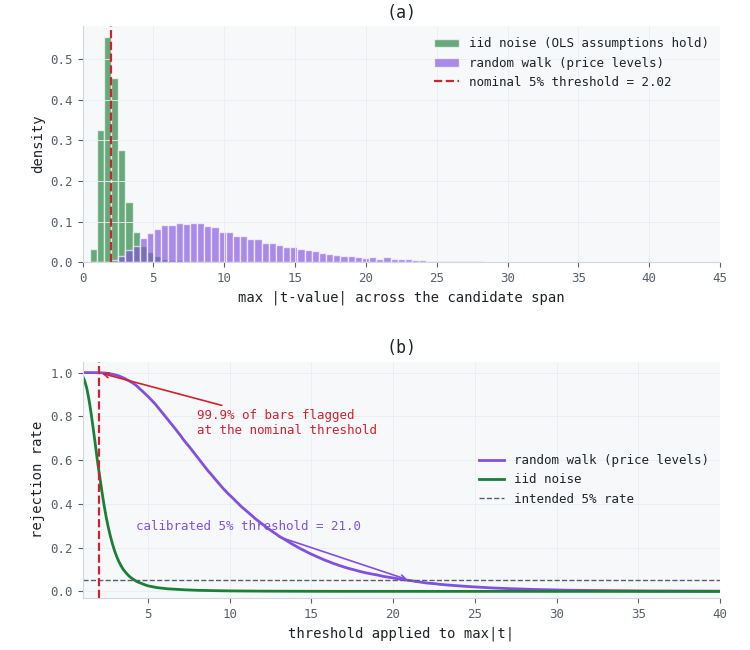
Figure 5. Two-panel illustration of the scan statistic under a null containing no trend

• Panel (a): distribution of the maximum absolute t-value across the candidate span for independent noise and for a random walk, against the nominal five percent threshold.
• Panel (b): fraction of trendless bars declared significant as a function of the threshold applied, with the calibrated five percent point marked.

Decomposing the inflation matters, because it determines the remedy. A single forty-bar window on a random walk already reaches a 95th percentile of 17.32. Scanning thirty-six windows and keeping the extreme raises that only to 21.04, a factor of about 1.21. Almost all the distortion comes from fitting a trend to an integrated series; only a small residual comes from searching over horizons. A multiple-testing adjustment on the horizon count, such as Bonferroni or Sidak, would therefore correct the smaller effect and leave the larger one in place.

Simulating the statistic that is actually reported is what works. Draw a driftless random walk of max(L) increments, compute the statistic on every trailing window in the span, keep the maximum, repeat a few thousand times, and take the upper quantiles as thresholds. Because the statistic at a bar depends only on the trailing max(L) observations, each replication needs no more history than that, which makes the whole calibration cheap enough to run once per configuration and cache.

Two caveats belong with this. A driftless random walk is a convenient null rather than a correct model of price, so what it produces is a calibration and not an exact test; a null with fat tails or volatility clustering would move the thresholds. And a calibrated threshold establishes only that the observed trend exceeds what a trendless series of the same length usually produces. It carries no implication about the next bar.

For labeling, none of this is fatal. Trend-scanning labels are used as a target, and a target that fires often is a class-balance problem rather than a validity problem — the earlier articles in this series that consume these labels are not affected by anything in this section. It becomes consequential the moment a t-value is used as a feature, compared against a fixed threshold, or read as evidence that a trend is real, which is exactly what get_trend_scanning_features invites and exactly why this correction belongs in this article rather than a note appended to Part 3.

Conclusion

Trend-scanning is unusual among the modules covered so far in this series because it already ships a correct causal mode; the risk is not a missing correction but an unmarked default. lookforward=True is right for labeling and wrong for features, and the function's signature gives no indication of which situation a caller is in. get_trend_scanning_features removes the choice rather than documenting it, by not exposing the parameter at all.

Two defects were measured directly rather than argued from the code. Calling the labeling default as a feature generator inflates a next-bar hit rate from 50% to as much as 61% on data with no real trend, with the visible size of the effect shrinking as the candidate horizon widens even though the underlying leak does not. Leaving the log transform on for a signed input series collapses 44.7% of bars to one constant value and flips the resulting sign on nearly a fifth of the output.

The reversal-and-reindex mechanism that makes the backward mode possible was checked directly against the forward output rather than trusted, and matched to floating-point precision.

Separately from the two defects above, the window-selection rule this module inherits from the published method compares t-values computed with different degrees of freedom. As a result, it may fail to select the most significant trend and may even report the opposite direction, a difference measured at 286x on the worked example. The t-value itself is inflated on price levels, to the point that 99.94% of bars in a trendless random walk exceed the nominal five percent threshold. Both corrections are supplied as an optional selection argument and a calibration routine rather than as changes to the default, so pipelines already built on this wrapper keep the behavior they were validated against.

The remaining article in this pair will port the causal feature set to MQL5, where the same forward/backward distinction has to be maintained without a reversible array to fall back on.

References

1. Lopez de Prado, M. Advances in Financial Machine Learning: Lecture 3/10.
2. Lopez de Prado, M. (2018). Advances in Financial Machine Learning. Wiley.
3. Lopez de Prado, M. (2020). Machine Learning for Asset Managers, Section 5.4. Cambridge University Press.
4. Granger, C. W. J. and Newbold, P. (1974). Spurious regressions in econometrics. Journal of Econometrics, 2(2), 111-120.

Attached Files

	File	Module	Description
1.	trend_scanning.py	afml.labeling	trend_scanning_labels and the Numba kernel _window_stats_numba, unmodified. Included for reference since get_trend_scanning_features calls it directly with lookforward=False.
2.	trend_scanning_features.py	afml.features.trend_scanning	get_trend_scanning_features: causal wrapper with no lookforward parameter, returning window, slope, t_value, rsquared.
3.	measure_leak.py	Verification	Next-bar hit-rate test on random-walk data, leaky versus causal mode, twenty seeds.
4.	horizon_sweep.py	Verification	Repeats the hit-rate test across six maximum-horizon settings; produces Figure 2(a).
5.	measure_log_defect.py	Verification	Quantifies the clip-and-log collapse on a signed mean-reverting series; produces Figure 2(b).
6.	trend_scanning_selection.py	afml.features.trend_scanning	Length-corrected window selection (select_horizon, signed_z) and random-walk threshold calibration (calibrate_threshold). Adds a selection argument to the wrapper rather than changing its default.
7.	MQL5.zip	Archive	All seven files above, unpacked to MQL5\Files\TrendScanningFeatures\. Extract with the MQL5 folder as the archive root directly into the terminal's data directory.