Bison Algorithm (BIA)

Contents

1. Introduction
2. Implementation of the algorithm
3. Test results

Introduction

In search of a better optimization method, this article introduces the Bison Algorithm (BIA), a swarm-inspired population-based optimization algorithm designed for solving continuous problems with a single objective function. The key features of BIA are two fundamental principles borrowed from the behavior of bison: the ability to move dynamically and a defensive strategy. The algorithm was developed by Czech researchers in 2017 and published in the Lecture Notes in Computer Science (Springer) in 2019. 

Bison are amazing animals with great endurance and strength. They are capable of developing high speed and maintaining it for half an hour. When surrounded by predators, they tend to form a circle, with the strongest individuals on the perimeter and the rest of the herd tending to move inside to take a safe position.

These two behavioral patterns were modeled in the Bison Algorithm and applied as an optimization technique. The first aspect, "speed and endurance," allows the algorithm's agents to explore the search space broadly, exploring new and potentially optimal areas. The second aspect, the "defensive circle," models a local search and stabilization mechanism, where agents gather around the most promising solutions, protecting them from premature rejection and refining their positions. Now let's see how this actually works in the algorithm.

Implementation of the algorithm

You are watching a herd of bison on the prairie. They need to find the best pasture with lush grass and clean water. But the prairie is huge! How do they do it? Let's divide the herd into two groups.

Main herd (80% of bison) consists of cautious animals. They stick together and move slowly in a group. "Security in numbers!" is their motto.

Explorers (20% of bison) are brave young animals. They run forward in one direction, exploring new territories. "What's there, behind the hill?" they think.

Two groups are formed: 40 bison from the main herd wander around a known area, and 10 runners gather near the fattest bison (it clearly knows where the richer grazing area is!) and prepare for the race. When a bison from the main herd moves to a new position, it first remembers where it stood. It takes several steps (from 0 to 3.5 meters). Then it tries the grass. If the new grass is worse, then it goes back. "A bird in the hand is worth two in the bush". If the runner-explorer finds a better place than the worst bison in the herd, then they swap places. Runners change direction slightly every day (10% to the left or right). This increases the chances of finding something new. When a herd gathers around the best bison, they do not simply cluster around the center. The leader (the fattest) has a "weight" of 100, the second - 90, the third - 80... the tenth - 10. 

Now imagine that:

• Pasture = solution search space
• Grass quality = objective function value
• Bison position = potential solution
• The best pasture = the optimal solution

The diagram below shows the initialization phase - the division of the population into a swarm group (80%) and a running group (20%). The main iteration loop consists of four steps: determining the swarm target (choosing between the best runner or the elite center), movement of the swarm group towards the center (weighted averaging of the elite center), movement of runners in the direction of research, checking and updating results.

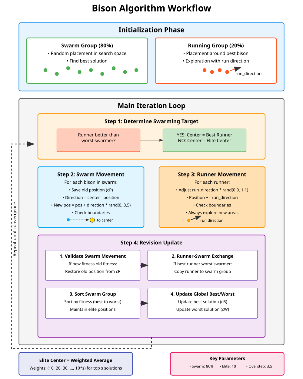
Figure 1. BIA algorithm workflow

Algorithm key parameters. Color scheme: green - swarm group, orange - running group, purple - checking and updating phase, blue - swarm movement. The arrows show the flow of execution and the directions of movement of the groups.

Let's start writing a pseudocode for the BIA algorithm.

INITIALIZATION:
1. Create a population of N bison
2. Divide into groups:
   - Swarm group (80%): Place randomly throughout the space
   - Running group (20%): Place around the best bison of the swarm group
3. Set a random running direction for scouts

MAIN CYCLE (repeat until convergence):
  
  SELECTING THE MOVEMENT GOAL:
  - IF the best of the running group has found a better place than the worst in the herd:
      Goal = position of the best of the running group
  - OTHERWISE:
      Target = weighted center of top 10 in herd
  
  SWARM GROUP MOVEMENT:
  - For each bison in the herd:
    1. Save current position
    2. Calculate the direction to the target
    3. Take a step towards the target (random length from 0 to 3.5)
    4. Check search area boundaries
  
  MOVEMENT OF THE RUNNING GROUP:
  - Change running direction slightly (×0.9-1.1)
  - For each individual:
    1. move in the direction of running
    2. check the boundaries of the search area
  
  ASSESSMENT AND UPDATE:
  1. Check the swarm group:
     - IF the new position is worse than the old one:
         Return to the old position
  
  2. Exchange between groups:
     - IF the best individual in a running group is better than the worst in the herd:
         Replace the worst in the herd with the best individual
  
  3. Sorting:
     - Sort the swarm group by quality
  
  4. Update:
     - Remember the best solution found
     - Remember the worst solution

CYCLE END

CALCULATION OF THE WEIGHTED CENTER:
- Take the 10 best solutions
- Assign weights: 1st gets weight 100, 2nd - 90, ..., 10th - 10
- Center = sum(position × weight) / sum(weights)

Now we have a better understanding of how everything works, and we can start writing the algorithm code. The class implements the Bison Algorithm and specifies inheritance from the C_AO base class.

Algorithm parameters:

• popSize — defines the total number of "individuals" or "agents" in the population participating in the algorithm.
• swarmGroupRate — specifies the proportion (in percent) of the total number of individuals that will make up the "swarm group".
• eliteGroupSize — defines the number of the very best individuals that form the "elite group" for calculating the center.
• overstep — sets the maximum step that a swarm group can take when moving.

The constructor sets default values for all parameters. The SetParams method allows updating the values of the algorithm parameters using data from an external source (represented by the "params" array).

Functionality:

• Init — method for initializing the algorithm using ranges of values for the parameters.
• Moving — method responsible for the movement or updating the state of individuals in a population.
• Revision — method used to revise and adjust the behavior of individuals or parameters.
• ComputeCenter — private method for computing the center of an elite group.
• CheckIfRunnerBetter — private method that checks whether any individual runner is better than others.

Internal variables:

• swarmGroupSize — calculated based on popSize and swarmGroupRate, determines the actual number of individuals in the swarm group.
• runningGroupSize — size of the running group (a subgroup in the overall population).
• runDirection — array that stores the direction of movement for each individual.
• center — array that stores the coordinates of the center of the elite group.

In general, the C_AO_BisonAlgorithm class is a block that implements a search strategy based on the concept of population, swarm and elite groups, and has configurable parameters.

class C_AO_BisonAlgorithm : public C_AO
{
  public: //----------------------------------------------------------
  ~C_AO_BisonAlgorithm () { }
  C_AO_BisonAlgorithm ()
  {
    ao_name = "BIA";
    ao_desc = "Bison Algorithm";
    ao_link = "https://www.mql5.com/en/articles/19444";

    popSize          = 50;    // population size
    swarmGroupRate   = 0.8;   // share of swarm group from population (80%)
    eliteGroupSize   = 10;    // size of the elite group for calculating the center (s parameter)
    overstep         = 3.5;   // maximum step of the swarm group

    ArrayResize (params, 4);

    params [0].name = "popSize";        params [0].val = popSize;
    params [1].name = "swarmGroupRate"; params [1].val = swarmGroupRate;
    params [2].name = "eliteGroupSize"; params [2].val = eliteGroupSize;
    params [3].name = "overstep";       params [3].val = overstep;
  }

  void SetParams ()
  {
    popSize        = (int)params [0].val;
    swarmGroupRate = params      [1].val;
    eliteGroupSize = (int)params [2].val;
    overstep       = params      [3].val;
  }

  bool Init (const double &rangeMinP  [],
             const double &rangeMaxP  [],
             const double &rangeStepP [],
             const int     epochsP = 0);

  void Moving   ();
  void Revision ();
  
  private:
  void ComputeCenter ();
  bool CheckIfRunnerBetter ();

  //------------------------------------------------------------------
  public:
  double swarmGroupRate;     // share of swarm group
  int    eliteGroupSize;     // size of the elite group (s parameter)
  double overstep;           // maximum step of the swarm group

  private: //---------------------------------------------------------
  int    swarmGroupSize;     // swarm group size
  int    runningGroupSize;   // running group size
  double runDirection [];    // running direction
  double center [];          // elite group center
};
//————————————————————————————————————————————————————————————————————

The Init method of the C_AO_BisonAlgorithm class is responsible for the initial configuration of the algorithm before it starts running. The method first attempts to perform a common, standardized initialization part, using the ranges of values for the parameters and the number of epochs passed to it. If this standard part fails, the entire initialization process is aborted. Next, based on the total population size and the given coefficient, the number of individuals that will belong to the "swarm group" is calculated. The remaining individuals form a "running group".

To ensure the correct operation of the algorithm, the sizes of these groups are checked. It is guaranteed that the swarm group will always have at least one member, and also that it will not occupy the entire population (leaving room for the running group). Similarly, it is verified that the elite group is not less than one and does not exceed the size of the swarm group, being its subset.

Memory is allocated for service arrays. The array used to store the direction of movement of individuals (for each dimension of the search space) and the array used to store the coordinates of the center of the elite group both arrays are resized to match the number of dimensions defined in the system. If all previous steps are completed successfully, the method returns "true" and the algorithm is ready to work.

//————————————————————————————————————————————————————————————————————
//--- Initialization
bool C_AO_BisonAlgorithm::Init (const double &rangeMinP  [],
                                const double &rangeMaxP  [],
                                const double &rangeStepP [],
                                const int     epochsP = 0)
{
  if (!StandardInit (rangeMinP, rangeMaxP, rangeStepP)) return false;

  //------------------------------------------------------------------
  // Calculate the sizes of groups
  swarmGroupSize   = (int)MathFloor (popSize * swarmGroupRate);
  runningGroupSize = popSize - swarmGroupSize;
  
  // Adjust group sizes
  if (swarmGroupSize < 1) swarmGroupSize = 1;
  if (swarmGroupSize >= popSize) swarmGroupSize = popSize - 1;
  if (eliteGroupSize < 1) eliteGroupSize = 1;
  if (eliteGroupSize > swarmGroupSize) eliteGroupSize = swarmGroupSize;
  
  // Initialize auxiliary arrays
  ArrayResize (runDirection, coords);
  ArrayResize (center, coords);

  return true;
}
//————————————————————————————————————————————————————————————————————

The Moving method of the C_AO_BisonAlgorithm class is the core of the algorithm, responsible for one iteration or step of population evolution. It consists of two main phases: the initial initialization of the population (if the algorithm is launched for the first time) and subsequent steps of updating the positions of individuals.

Phase 1: Initial initialization (first run): If the algorithm is run for the first time (the "revision" flag is set to 'false'), the following sequence of actions is performed:

• Swarm group generation. Individuals included in the swarm group are initialized with random values within the ranges specified for each parameter. Once generated, these values can be further adjusted to comply with the parameter discretization step.
• Searching for the best bison. Among all the individuals in a swarm group, there is one that has the best fitness (the highest value of the objective function).
• Running group generation. The remaining individuals of the population (the running group) are initialized around the best bison found. Their positions are generated randomly in some neighborhood of the best solution, and then also adjusted in accordance with the ranges and steps of the parameters.
• Initialization of the movement direction vector. For each dimension of the search space, a random movement direction vector is generated. The magnitude of this vector depends on the overall range of parameter values, and its sign (positive or negative) is also chosen randomly.
• Set the initialization flag. The "revision" flag is set to 'true', the initialization is complete, and only update steps will be performed from now on.

Phase 2: Main iteration cycle (next steps): Once the initialization has been performed, the method performs the following steps for each iteration:

Determining the swarm target. The algorithm checks whether any solution from the running group is better than the current "swarming target".

• If the solution from the running group turns out to be better, then this swarming goal (centroid) is set equal to this better solution.
• Otherwise, a new centroid is calculated, which represents a weighted center of the best solutions in the population.

Swarm group movement. Each individual in the swarm group moves.

• First, the current positions and fitness values of the individual are saved.
• The new position is then calculated by moving from the current position towards the target swarming point. The magnitude of this movement is determined by a random factor that regulates the "stepping" over the target.
• The resulting new position is then adjusted to stay within the acceptable ranges and take into account the parameter step.

Correction of the movement direction vector. The direction vector used by the running group varies slightly randomly. This adds some variety to the runners' movements.

Running group movement. Each individual in the running group moves using adjusted direction vector.

• The new position is calculated by adding the direction vector to the current position.
• This new position is then adjusted to stay within the acceptable ranges and take into account the parameter step.

Thus, the Moving method models the behavior of a group of individuals: part of the group (the swarm) moves toward a common goal, responding to the best solutions, and the other part (the running) follows the adjusted direction vector, which can also change.

/————————————————————————————————————————————————————————————————————
//--- Main step of the algorithm
void C_AO_BisonAlgorithm::Moving ()
{
  // Starting initialization of the population
  if (!revision)
  {
    // Generate a swarm group randomly
    for (int i = 0; i < swarmGroupSize; i++)
    {
      for (int j = 0; j < coords; j++)
      {
        a [i].c [j] = u.RNDfromCI (rangeMin [j], rangeMax [j]);
        a [i].c [j] = u.SeInDiSp (a [i].c [j], rangeMin [j], rangeMax [j], rangeStep [j]);
      }
    }
    
    // Find the best solution among the swarm group to initialize the runners
    int bestIdx = 0;
    double bestFit = a [0].f;
    for (int i = 1; i < swarmGroupSize; i++)
    {
      if (a [i].f > bestFit)
      {
        bestFit = a [i].f;
        bestIdx = i;
      }
    }
    
    // Generate a running group around the best bison
    double neighbourhood = (rangeMax [0] - rangeMin [0]) / 15.0;
    for (int i = swarmGroupSize; i < popSize; i++)
    {
      for (int j = 0; j < coords; j++)
      {
        a [i].c [j] = a [bestIdx].c [j] + u.RNDfromCI (-neighbourhood, neighbourhood);
        a [i].c [j] = u.SeInDiSp (a [i].c [j], rangeMin [j], rangeMax [j], rangeStep [j]);
      }
    }
    
    // Generate run direction = random((ub-lb)/45, (ub-lb)/15)
    for (int j = 0; j < coords; j++)
    {
      double range = rangeMax [j] - rangeMin [j];
      runDirection [j] = u.RNDfromCI (range / 45.0, range / 15.0);
      if (u.RNDprobab () < 0.5) runDirection [j] = -runDirection [j];
    }
    
    revision = true;
    return;
  }

  //------------------------------------------------------------------
  // Main iteration loop
  
  // 1. Define swarming target
  if (CheckIfRunnerBetter ())
  {
    // If runner is better than swarmer, center = runner
    // center is already set in CheckIfRunnerBetter
  }
  else
  {
    // Otherwise, calculate the center of the strongest solutions
    ComputeCenter ();
  }
  
  // 2. Swarm group movement
  for (int i = 0; i < swarmGroupSize; i++)
  {
    // Save old positions in cP and fitness in fP
    ArrayCopy (a [i].cP, a [i].c, 0, 0, coords);
    a [i].fP = a [i].f;
    
    // Calculate a new candidate for the position
    for (int c = 0; c < coords; c++)
    {
      double direction = center [c] - a [i].c [c];
      a [i].c [c] = a [i].c [c] + direction * u.RNDfromCI (0.0, overstep);
      a [i].c [c] = u.SeInDiSp (a [i].c [c], rangeMin [c], rangeMax [c], rangeStep [c]);
    }
  }
  
  // 3. Correction of the vector 'run direction'
  for (int j = 0; j < coords; j++)
  {
    runDirection [j] = runDirection [j] * u.RNDfromCI (0.9, 1.1);
  }
  
  // 4. Running group movement
  for (int i = swarmGroupSize; i < popSize; i++)
  {
    for (int c = 0; c < coords; c++)
    {
      a [i].c [c] = a [i].c [c] + runDirection [c];
      a [i].c [c] = u.SeInDiSp (a [i].c [c], rangeMin [c], rangeMax [c], rangeStep [c]);
    }
  }
}
//————————————————————————————————————————————————————————————————————

Revision method of the C_AO_BisonAlgorithm class is meant for updating the state of the population after completing one step of movement and assessing the fitness of individuals, as well as for summing up the results of the iteration.

Swarm group correction. For each individual in the swarm group, it is checked whether its new position (calculated in the previous step) is better than its previous (saved) position. If the new position is worse, the individual returns to its previous, better position. In this way, individuals of the swarm group do not worsen their results.

Comparing a running group with a swarm:

• The best individual in the running group (with the highest fitness) and the worst individual in a swarm group (with the lowest fitness).
• If the best individual from the running group turns out to be better than the worse the individual from the swarm group, the worse the individual from the swarm group is replaced with the best individual from the running group. This allows stronger solutions from the running group to enter the swarm group.

Sorting the swarm group:

• A temporary copy of all individuals in the swarm group is created.
• This temporary copy is sorted in descending order of fitness (from best to worst).
• After sorting, individuals from the sorted temporary copy are copied back to the general population. This ensures that the swarm group will always contain the best solutions found so far.

Global solutions update:

• Best global solution. The fitness of the best individual in the swarm group (which is now the best solution after sorting) is compared with the current best global solution. If the best individual of the swarm group is better, the global best solution is updated.
• Worst global solution. All individuals in the population (both swarming and running) are then examined to find the weakest one. If an individual is found with a fitness value lower than the current worst global solution, the worst global solution is updated.

Thus, the Revision method serves as the result-processing stage that selects the best solutions, maintains order and updates in the swarm group, and tracks the overall progress of the algorithm, storing the best and worst solutions found.

//————————————————————————————————————————————————————————————————————
//--- Update and check results
void C_AO_BisonAlgorithm::Revision ()
{
  // 1. For a swarm group: update positions only if the new position is better
  for (int i = 0; i < swarmGroupSize; i++)
  {
    // If the new position is worse than the old one, return the old one
    if (a [i].f < a [i].fP)
    {
      ArrayCopy (a [i].c, a [i].cP, 0, 0, coords);
      a [i].f = a [i].fP;
    }
  }
  
  // 2. Let's check if runner has found a better solution than swarmer
  double bestRunnerFitness = -DBL_MAX;
  int bestRunnerIdx = -1;
  double worstSwarmerFitness = DBL_MAX;
  int worstSwarmerIdx = -1;
  
  for (int i = swarmGroupSize; i < popSize; i++)
  {
    if (a[i].f > bestRunnerFitness)
    {
      bestRunnerFitness = a[i].f;
      bestRunnerIdx = i;
    }
  }
  
  for (int i = 0; i < swarmGroupSize; i++)
  {
    if (a[i].f < worstSwarmerFitness)
    {
      worstSwarmerFitness = a[i].f;
      worstSwarmerIdx = i;
    }
  }
  
  // If the runner is better than the worst swarmer, copy the runner to the swarming group
  if (bestRunnerIdx >= 0 && worstSwarmerIdx >= 0 && bestRunnerFitness > worstSwarmerFitness)
  {
    ArrayCopy (a[worstSwarmerIdx].c, a[bestRunnerIdx].c, 0, 0, coords);
    a[worstSwarmerIdx].f = a[bestRunnerIdx].f;
  }
  
  // 3. Sort the swarm group
  // Create a temporary array to sort only the swarm group
  S_AO_Agent swarmTemp [];
  ArrayResize (swarmTemp, swarmGroupSize);
  
  // Copy the swarm group
  for (int i = 0; i < swarmGroupSize; i++)
  {
    swarmTemp[i].Init(coords);
    ArrayCopy (swarmTemp[i].c, a[i].c, 0, 0, coords);
    swarmTemp[i].f = a[i].f;
    ArrayCopy (swarmTemp[i].cP, a[i].cP, 0, 0, coords);
    swarmTemp[i].fP = a[i].fP;
  }
  
  // Sort
  S_AO_Agent tempSorted [];
  ArrayResize (tempSorted, swarmGroupSize);
  u.Sorting (swarmTemp, tempSorted, swarmGroupSize);
  
  // Copy the swarm group sorted back
  for (int i = 0; i < swarmGroupSize; i++)
  {
    ArrayCopy (a[i].c, swarmTemp[i].c, 0, 0, coords);
    a[i].f = swarmTemp[i].f;
    ArrayCopy (a[i].cP, swarmTemp[i].cP, 0, 0, coords);
    a[i].fP = swarmTemp[i].fP;
  }
  
  // 4. Update the global best and worst case solution
  if (a[0].f > fB)
  {
    fB = a[0].f;
    ArrayCopy (cB, a[0].c, 0, 0, WHOLE_ARRAY);
  }
  
  // Find the worst in the entire population
  for (int i = 0; i < popSize; i++)
  {
    if (a[i].f < fW)
    {
      fW = a[i].f;
      ArrayCopy (cW, a[i].c, 0, 0, WHOLE_ARRAY);
    }
  }
}
//————————————————————————————————————————————————————————————————————

The CheckIfRunnerBetter method is used to determine whether the running group contains a more promising solution than those present in the swarm group. If such a solution is found, it becomes a new "target" for swarming.

Search for the best "runner". The method first scans all individuals that belong to the "running group" (not part of the swarm). It finds the individual with the best fitness (the highest objective function value) among all runners and stores its index and fitness value.

Search for the worst "swarm". The method then analyzes the individuals that make up the "swarm group". It finds the individual with the worst fitness (the lowest value of the objective function) among the swarm.

Comparing and goal determination. After this, a comparison takes place:

• If the best runner has a fitness higher than the worst swarm, this means that the running group has indeed found a better solution.
• In this case, the position (coordinates) of the best "runner" is assigned to a variable denoting the "center" or "swarming target". The method returns a value indicating that the swarming target has been updated.

Returning the result:

• If the best "runner" is better than the worst individual in the "swarm", the method reports this by returning an affirmative value.
• Otherwise (if no "runner" has surpassed the worst "swarm" member), the method reports this by returning a negative value, and the swarm center remains the same.

This method thus allows for dynamic changes in the search direction: if stronger solutions emerge in the "exploratory" running group, they become a guide for the "social" swarm group.

//————————————————————————————————————————————————————————————————————
//--- Check whether a runner is better than a swarmer
bool C_AO_BisonAlgorithm::CheckIfRunnerBetter ()
{
  // Find the best runner
  double bestRunnerFitness = -DBL_MAX;
  int bestRunnerIdx = -1;
  
  for (int i = swarmGroupSize; i < popSize; i++)
  {
    if (a[i].f > bestRunnerFitness)
    {
      bestRunnerFitness = a[i].f;
      bestRunnerIdx = i;
    }
  }
  
  // Find the worst swarmer 
  double worstSwarmerFitness = DBL_MAX;
  
  for (int i = 0; i < swarmGroupSize; i++)
  {
    if (a[i].f < worstSwarmerFitness)
    {
      worstSwarmerFitness = a[i].f;
    }
  }
  
  // If the runner is better than the swarmer, set it as the center
  if (bestRunnerIdx >= 0 && bestRunnerFitness > worstSwarmerFitness)
  {
    ArrayCopy (center, a[bestRunnerIdx].c, 0, 0, coords);
    return true;
  }
  
  return false;
}
//————————————————————————————————————————————————————————————————————

The ComputeCenter method calculates a new "target" position (center) for the swarm group based on the best solutions found. Here is how it works:

• Reset the target position. First, all components of the future target position (center) are reset to zero. This prepares them to accumulate new values.
• Determine the number of best solutions. The method selects exactly how many best solutions will be used to calculate the center. It takes the minimum value of two parameters:

• eliteGroupSize — maximum number of "elite" solutions that can be taken into account;
• swarmGroupSize — size of the current swarm group;
• This ensures that we use either all given elite solutions, or as many as there are in the swarm group if there are fewer elite solutions.
• Assigning weights. A set of weights is created for each of the selected best solutions. These weights increase linearly: the first solution receives less weight, the second one receives more, and so on, until the last one. Specifically, the weights are set as 10, 20, 30... up to s * 10, where s is the number of best solutions taken into account. These weights indicate how significant each decision is when calculating the center.
• Accumulation of the total sum of weights. All calculated weights are summed up. This total amount will be needed for normalization.
• Weighted summation of positions. Now for each dimension (coordinate) of the position:
• the value of the corresponding coordinate is taken from each of the s best solutions;
• this coordinate value is multiplied by the weight of the corresponding best solution. It is important to note that the weights are applied in reverse order: the best solution (the first in the sorted list) gets the largest weight, the second gets the next largest, and so on.
• the results of these multiplications for all s best solutions are summed for a given coordinate.
• Normalization. The resulting sum of weighted coordinates for each dimension is divided by the total sum of all weights. This makes the calculation a "weighted average", ensuring that the final position of the center is in some "middle" region of the best solutions found, with higher quality solutions having a greater influence.

As a result, the ComputeCenter method creates a new "target" position, which is a kind of "average" best solution, but with a preference for the highest quality ones, which helps guide the further search of the swarm.

//————————————————————————————————————————————————————————————————————
//--- Calculate the center of the elite group
void C_AO_BisonAlgorithm::ComputeCenter ()
{
  // Reset the center
  for (int j = 0; j < coords; j++)
  {
    center [j] = 0.0;
  }
  
  // Calculate the weighted center from the s best solutions
  double weights [];
  int s = MathMin(eliteGroupSize, swarmGroupSize);
  ArrayResize (weights, s);
  double totalWeight = 0.0;
  
  // weight = (10, 20, 30, ..., 10*s)
  for (int i = 0; i < s; i++)
  {
    weights[i] = (i + 1) * 10.0;
    totalWeight += weights[i];
  }
  
  // center = sum(weight[i] * position[i]) / sum(weights)
  for (int j = 0; j < coords; j++)
  {
    for (int i = 0; i < s; i++)
    {
      center[j] += (weights[s - 1 - i] * a[i].c[j]) / totalWeight;
    }
  }
}
//————————————————————————————————————————————————————————————————————

Test results

As we can see, the results are average; on the discrete Megacity function they are slightly lower; the algorithm has more difficulty coping with discrete problems.

Bison|Bison Algorithm|50.0|0.8|10|3.5|
=============================
5 Hilly's; Func runs: 10000; result: 0.761847128451914
25 Hilly's; Func runs: 10000; result: 0.4002698460741261
500 Hilly's; Func runs: 10000; result: 0.25201531651422443
=============================
5 Forest's; Func runs: 10000; result: 0.7620992740937584
25 Forest's; Func runs: 10000; result: 0.45225292646780135
500 Forest's; Func runs: 10000; result: 0.19295587559803248
=============================
5 Megacity's; Func runs: 10000; result: 0.48769230769230765
25 Megacity's; Func runs: 10000; result: 0.19876923076923075
500 Megacity's; Func runs: 10000; result: 0.10058461538461608
=============================
All score: 3.60849 (40.09%)

The visualization of the BIA algorithm performance shows a fairly large spread of results not only for low-dimensional functions (green lines), but also for medium-dimensional functions (blue lines).

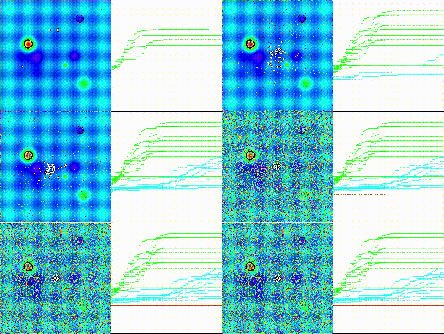
BIA on the Hilly test function

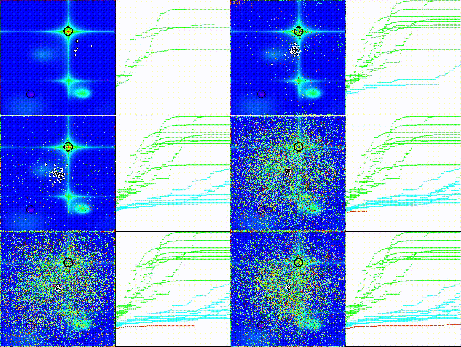
BIA on the Forest test function

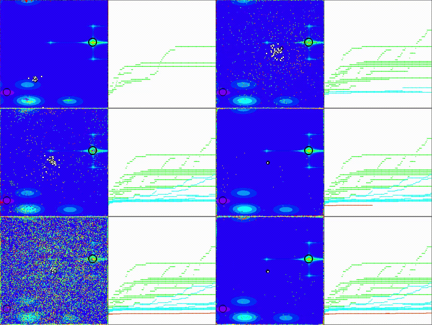
BIA on the Megacity test function

The BIA algorithm is presented for informational purposes in the rating table of population optimization methods.

#	AO	Description	Hilly			Hilly Final	Forest			Forest Final	Megacity (discrete)			Megacity Final	Final Result	% of MAX
			10 p (5 F)	50 p (25 F)	1000 p (500 F)		10 p (5 F)	50 p (25 F)	1000 p (500 F)		10 p (5 F)	50 p (25 F)	1000 p (500 F)
1	DOAdingom	dingo_optimization_algorithm_M	0.47968	0.45367	0.46369	1.39704	0.94145	0.87909	0.91454	2.73508	0.78615	0.86061	0.84805	2.49481	6.627	73.63
1	ANS	across neighbourhood search	0.94948	0.84776	0.43857	2.23581	1.00000	0.92334	0.39988	2.32323	0.70923	0.63477	0.23091	1.57491	6.134	68.15
2	CLA	code lock algorithm (joo)	0.95345	0.87107	0.37590	2.20042	0.98942	0.91709	0.31642	2.22294	0.79692	0.69385	0.19303	1.68380	6.107	67.86
3	AMOm	animal migration ptimization M	0.90358	0.84317	0.46284	2.20959	0.99001	0.92436	0.46598	2.38034	0.56769	0.59132	0.23773	1.39675	5.987	66.52
4	(P+O)ES	(P+O) evolution strategies	0.92256	0.88101	0.40021	2.20379	0.97750	0.87490	0.31945	2.17185	0.67385	0.62985	0.18634	1.49003	5.866	65.17
5	CTA	comet tail algorithm (joo)	0.95346	0.86319	0.27770	2.09435	0.99794	0.85740	0.33949	2.19484	0.88769	0.56431	0.10512	1.55712	5.846	64.96
6	TETA	time evolution travel algorithm (joo)	0.91362	0.82349	0.31990	2.05701	0.97096	0.89532	0.29324	2.15952	0.73462	0.68569	0.16021	1.58052	5.797	64.41
7	SDSm	stochastic diffusion search M	0.93066	0.85445	0.39476	2.17988	0.99983	0.89244	0.19619	2.08846	0.72333	0.61100	0.10670	1.44103	5.709	63.44
8	BOAm	billiards optimization algorithm M	0.95757	0.82599	0.25235	2.03590	1.00000	0.90036	0.30502	2.20538	0.73538	0.52523	0.09563	1.35625	5.598	62.19
9	AAm	archery algorithm M	0.91744	0.70876	0.42160	2.04780	0.92527	0.75802	0.35328	2.03657	0.67385	0.55200	0.23738	1.46323	5.548	61.64
10	ESG	evolution of social groups (joo)	0.99906	0.79654	0.35056	2.14616	1.00000	0.82863	0.13102	1.95965	0.82333	0.55300	0.04725	1.42358	5.529	61.44
11	SIA	simulated isotropic annealing (joo)	0.95784	0.84264	0.41465	2.21513	0.98239	0.79586	0.20507	1.98332	0.68667	0.49300	0.09053	1.27020	5.469	60.76
12	EOm	extremal_optimization_M	0.76166	0.77242	0.31747	1.85155	0.99999	0.76751	0.23527	2.00277	0.74769	0.53969	0.14249	1.42987	5.284	58.71
13	BBO	biogeography based optimization	0.94912	0.69456	0.35031	1.99399	0.93820	0.67365	0.25682	1.86867	0.74615	0.48277	0.17369	1.40261	5.265	58.50
14	ACS	artificial cooperative search	0.75547	0.74744	0.30407	1.80698	1.00000	0.88861	0.22413	2.11274	0.69077	0.48185	0.13322	1.30583	5.226	58.06
15	DA	dialectical algorithm	0.86183	0.70033	0.33724	1.89940	0.98163	0.72772	0.28718	1.99653	0.70308	0.45292	0.16367	1.31967	5.216	57.95
16	BHAm	black hole algorithm M	0.75236	0.76675	0.34583	1.86493	0.93593	0.80152	0.27177	2.00923	0.65077	0.51646	0.15472	1.32195	5.196	57.73
17	ASO	anarchy society optimization	0.84872	0.74646	0.31465	1.90983	0.96148	0.79150	0.23803	1.99101	0.57077	0.54062	0.16614	1.27752	5.178	57.54
18	RFO	royal flush optimization (joo)	0.83361	0.73742	0.34629	1.91733	0.89424	0.73824	0.24098	1.87346	0.63154	0.50292	0.16421	1.29867	5.089	56.55
19	AOSm	atomic orbital search M	0.80232	0.70449	0.31021	1.81702	0.85660	0.69451	0.21996	1.77107	0.74615	0.52862	0.14358	1.41835	5.006	55.63
20	TSEA	turtle shell evolution algorithm (joo)	0.96798	0.64480	0.29672	1.90949	0.99449	0.61981	0.22708	1.84139	0.69077	0.42646	0.13598	1.25322	5.004	55.60
21	BSA	backtracking_search_algorithm	0.97309	0.54534	0.29098	1.80941	0.99999	0.58543	0.21747	1.80289	0.84769	0.36953	0.12978	1.34700	4.959	55.10
22	DE	differential evolution	0.95044	0.61674	0.30308	1.87026	0.95317	0.78896	0.16652	1.90865	0.78667	0.36033	0.02953	1.17653	4.955	55.06
23	SRA	successful restaurateur algorithm (joo)	0.96883	0.63455	0.29217	1.89555	0.94637	0.55506	0.19124	1.69267	0.74923	0.44031	0.12526	1.31480	4.903	54.48
24	CRO	chemical reaction optimization	0.94629	0.66112	0.29853	1.90593	0.87906	0.58422	0.21146	1.67473	0.75846	0.42646	0.12686	1.31178	4.892	54.36
25	BIO	blood inheritance optimization (joo)	0.81568	0.65336	0.30877	1.77781	0.89937	0.65319	0.21760	1.77016	0.67846	0.47631	0.13902	1.29378	4.842	53.80
26	DOA	dream_optimization_algorithm	0.85556	0.70085	0.37280	1.92921	0.73421	0.48905	0.24147	1.46473	0.77231	0.47354	0.18561	1.43146	4.825	53.62
27	BSA	bird swarm algorithm	0.89306	0.64900	0.26250	1.80455	0.92420	0.71121	0.24939	1.88479	0.69385	0.32615	0.10012	1.12012	4.809	53.44
28	DEA	dolphin_echolocation_algorithm	0.75995	0.67572	0.34171	1.77738	0.89582	0.64223	0.23941	1.77746	0.61538	0.44031	0.15115	1.20684	4.762	52.91
29	HS	harmony search	0.86509	0.68782	0.32527	1.87818	0.99999	0.68002	0.09590	1.77592	0.62000	0.42267	0.05458	1.09725	4.751	52.79
30	SSG	saplings sowing and growing	0.77839	0.64925	0.39543	1.82308	0.85973	0.62467	0.17429	1.65869	0.64667	0.44133	0.10598	1.19398	4.676	51.95
31	BCOm	bacterial chemotaxis optimization M	0.75953	0.62268	0.31483	1.69704	0.89378	0.61339	0.22542	1.73259	0.65385	0.42092	0.14435	1.21912	4.649	51.65
32	ABO	african buffalo optimization	0.83337	0.62247	0.29964	1.75548	0.92170	0.58618	0.19723	1.70511	0.61000	0.43154	0.13225	1.17378	4.634	51.49
33	(PO)ES	(PO) evolution strategies	0.79025	0.62647	0.42935	1.84606	0.87616	0.60943	0.19591	1.68151	0.59000	0.37933	0.11322	1.08255	4.610	51.22
34	FBA	fractal-based Algorithm	0.79000	0.65134	0.28965	1.73099	0.87158	0.56823	0.18877	1.62858	0.61077	0.46062	0.12398	1.19537	4.555	50.61
35	TSm	tabu search M	0.87795	0.61431	0.29104	1.78330	0.92885	0.51844	0.19054	1.63783	0.61077	0.38215	0.12157	1.11449	4.536	50.40
36	BSO	brain storm optimization	0.93736	0.57616	0.29688	1.81041	0.93131	0.55866	0.23537	1.72534	0.55231	0.29077	0.11914	0.96222	4.498	49.98
37	WOAm	wale optimization algorithm M	0.84521	0.56298	0.26263	1.67081	0.93100	0.52278	0.16365	1.61743	0.66308	0.41138	0.11357	1.18803	4.476	49.74
38	AEFA	artificial electric field algorithm	0.87700	0.61753	0.25235	1.74688	0.92729	0.72698	0.18064	1.83490	0.66615	0.11631	0.09508	0.87754	4.459	49.55
39	AEO	artificial ecosystem-based optimization algorithm	0.91380	0.46713	0.26470	1.64563	0.90223	0.43705	0.21400	1.55327	0.66154	0.30800	0.28563	1.25517	4.454	49.49
40	CAm	camel algorithm M	0.78684	0.56042	0.35133	1.69859	0.82772	0.56041	0.24336	1.63149	0.64846	0.33092	0.13418	1.11356	4.444	49.37
41	ACOm	ant colony optimization M	0.88190	0.66127	0.30377	1.84693	0.85873	0.58680	0.15051	1.59604	0.59667	0.37333	0.02472	0.99472	4.438	49.31
42	CMAES	covariance_matrix_adaptation_evolution_strategy	0.76258	0.72089	0.00000	1.48347	0.82056	0.79616	0.00000	1.61672	0.75846	0.49077	0.00000	1.24923	4.349	48.33
43	DA_duelist	duelist_algorithm	0.92782	0.53778	0.27792	1.74352	0.86957	0.47536	0.18193	1.52686	0.62153	0.33569	0.11715	1.07437	4.345	48.28
44	BFO-GA	bacterial foraging optimization - ga	0.89150	0.55111	0.31529	1.75790	0.96982	0.39612	0.06305	1.42899	0.72667	0.27500	0.03525	1.03692	4.224	46.93
	BIA	bison_algorithm	0.76185	0.40027	0.25201	1.41413	0.76210	0.45225	0.19296	1.40731	0.48769	0.19877	0.10058	0.78704	3.608	40.09
	RW	random walk	0.48754	0.32159	0.25781	1.06694	0.37554	0.21944	0.15877	0.75375	0.27969	0.14917	0.09847	0.52734	2.348	26.09

Summary

The Bison Algorithm introduces an interesting concept of the explorer/exploiter divide, but in its current implementation it is inferior to modern metaheuristics. The main value lies in the idea of a clear separation of roles, which can be successfully integrated into hybrid approaches. 

Test results show that the algorithm performs averagely, failing to reach the level of top metaheuristics, and has difficulty solving discrete problems. To get into the rating table, significant improvements to the movement mechanisms and adaptation of parameters are required. The algorithm can be used in problems where simplicity of implementation and interpretability are important, but maximum accuracy is not required.

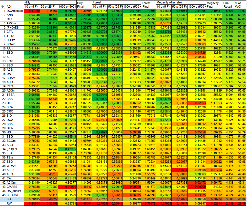
Figure 2. Color-coded comparison of algorithms across the corresponding tests

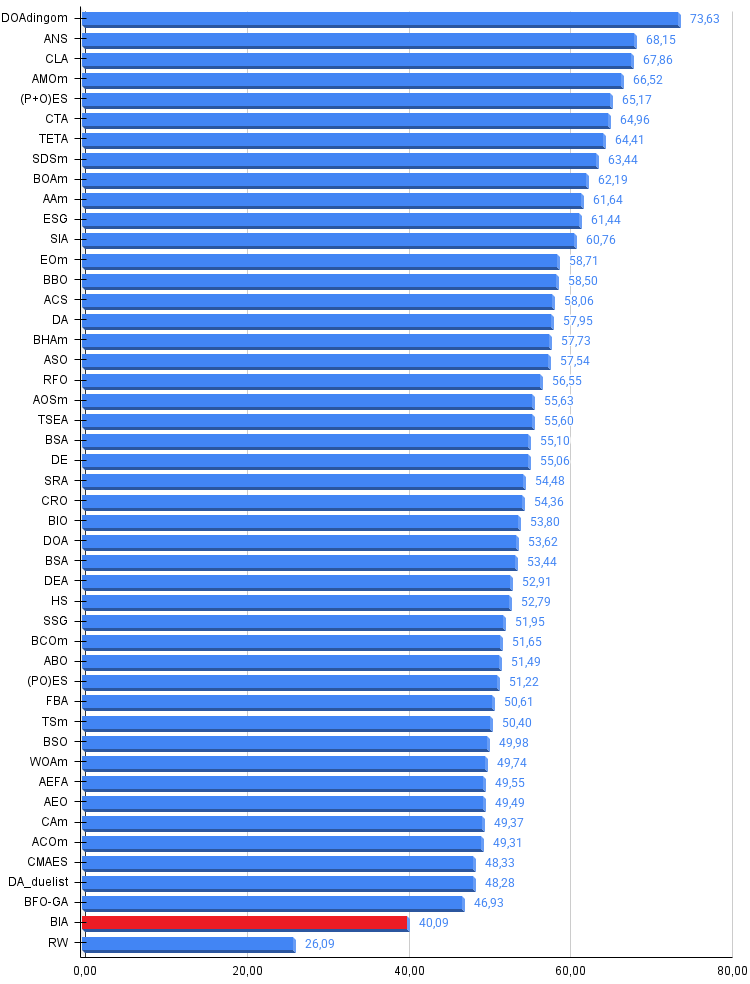
Figure 3. Histogram of algorithm testing results (scale from 0 to 100, the higher the better, where 100 is the maximum possible theoretical result, in the archive there is a script for calculating the rating table)

BIA pros and cons:

Pros:

1. Simple implementation.
2. Fast.

Cons:

1. High variability on low- and medium-dimensional test functions.

The article is accompanied by an archive with the current versions of the algorithm codes. The author of the article is not responsible for the absolute accuracy in the description of canonical algorithms. Changes have been made to many of them to improve search capabilities. The conclusions and judgments presented in the articles are based on the results of the experiments.

• github: https://github.com/JQSakaJoo/Population-optimization-algorithms-MQL5

Programs used in the article

#	Name	Type	Description
1	#C_AO.mqh	Include	Parent class of population optimization algorithms
2	#C_AO_enum.mqh	Include	Enumeration of population optimization algorithms
3	TestFunctions.mqh	Include	Library of test functions
4	TestStandFunctions.mqh	Include	Test stand function library
5	Utilities.mqh	Include	Library of auxiliary functions
6	CalculationTestResults.mqh	Include	Script for calculating results for the comparison table
7	Testing AOs.mq5	Script	The unified test stand for all population optimization algorithms
8	Simple use of population optimization algorithms.mq5	Script	A simple example of using population optimization algorithms without visualization
9	Test_AO_BIA.mq5	Script	BIA test stand