Mapping the Shape of Price: The Mapper Lens and Cover in MQL5

Contents

1. Introduction: A Second Way to See a Cloud
2. The Output of This Article
3. What Mapper Does in Four Steps
4. The Lens: One Number per Point
5. Implementation: CTDAMapperFilter
6. The Cover: Overlapping Intervals
7. Implementation: CTDAMapperCover
8. The Demo Script
9. What's Next
10. Conclusion

Introduction: A Second Way to See a Cloud

Earlier in this series, we embedded a price series into a point cloud and summarized its shape with a persistence diagram. A diagram is a precise object. It is also an abstract one. It tells you a loop exists and how strong it is, but it does not draw you a picture of the cloud you can point at and read.

The Mapper algorithm gives you that picture. It takes the same point cloud and compresses it into a small graph: a handful of nodes joined by edges. A round cloud becomes a ring of nodes. A branching cloud becomes a tree. A cloud in two separated pieces becomes two disconnected clusters. You look at the graph and you see the structure directly.

For a trader, the appeal is direct. A persistence diagram answers a yes-or-no question about whether structure is present. A Mapper graph shows you that structure itself, laid out as a shape you can compare from one window to the next: a clean ring reads differently at a glance from a fragmented chain or two disconnected pieces. That picture is a lossy compression, though, and its quality depends entirely on a few choices made at the very start: which one-dimensional summary of the cloud to use, how finely to slice it, and how much the slices overlap. Choose them well and the graph reveals real structure. Choose them badly and no clustering later can recover it. Getting those choices right, and checking that they are right, is the subject of this article.

So this article deliberately stops before the graph. It builds no node and no edge. Its goal is narrow and testable: produce the two artifacts the graph step will need, and hand you simple checks that confirm they are correct before you go further. The first artifact is a lens, one scalar value f[i] for every point, together with the minimum, maximum, and range of those values. The second is a cover, a set of evenly spaced overlapping intervals that slice the lens range, each carrying the list of point indices that fall inside it. Both are built on two objects from earlier in the series, a point cloud and its pairwise distance matrix, covered in an earlier article. We reuse those two classes here without rebuilding them. The intrinsic lenses read the whole distance matrix and so cost order N squared, but they only read distances already computed, never recompute them. The coordinate lens is cheaper and depends on the frame you pick.

The checks matter as much as the artifacts. The first guards against a degenerate lens. A lens that returns the same value for every point has a range of zero, and a zero range cannot be sliced into meaningful intervals, so the cover correctly collapses to a single bin. That is not a bug. It is what a symmetric cloud does to an intrinsic lens, and spotting it is the first thing to verify. The second check confirms the overlap: when the gain is positive, the member counts summed across all intervals exceed N, because points in the overlap are counted twice. The demo prints the log output both checks read from, and the article recommends starting values for the two cover parameters, a resolution of roughly 5 to 15 and a gain of roughly 0.2 to 0.5.

The Output of This Article

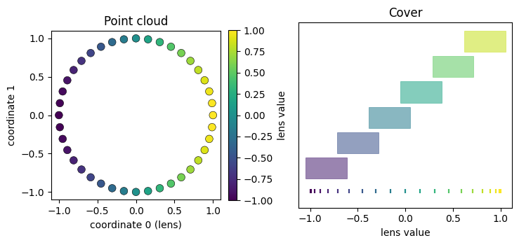
Fig. 1. A price cloud, here a circle, colored by the coordinate lens (left), and the six overlapping cover intervals its value range is sliced into (right). Every point falls into one or two intervals.

The cloud above is a circle. Each point carries a color set by the lens, in this case the value of the first coordinate. The bands beside it are the cover: six intervals along the value axis, each overlapping its neighbors. Every point falls into one or two bands, depending on where its color lands.

That pairing, a value per point and a set of overlapping bins, is the whole output of this article. The next article groups the points inside each band and connects the groups into a graph. For now, the goal is to produce the lens and the cover correctly, and to understand why the choice of lens matters as much as it does.

What Mapper Does in Four Steps

Mapper turns a point cloud into a graph in four steps. It helps to see all four before we build the first two.

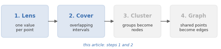
Fig. 2. The four steps of the Mapper pipeline. This article builds the first two, the lens and the cover; clustering and the graph follow in the next article.

1. Lens. Assign one number to every point. This projects the cloud onto a single axis of your choosing.
2. Cover. Slice the range of that number into overlapping intervals. Each point lands in one or more intervals.
3. Cluster. Inside each interval, group points that are close together in the original cloud. Each group becomes a node.
4. Graph. Join two nodes with an edge when they share points. The overlap between intervals is what creates the shared points, and so the edges.

This article covers steps one and two. Steps three and four are the subject of the next article. The clustering and graph classes exist in the attached library, but we treat them as black boxes here and say nothing about how they work until then.

The reason to split the work this way is that the first two steps are where all the parameter sensitivity lives. If the lens is a poor summary of the cloud, no amount of clever clustering later will recover the structure. A good lens and a sensible cover are most of the battle. The rest of this article builds them.

The Lens: One Number per Point

A lens is a function that maps each point of the cloud to a single real number. It is the axis Mapper looks along. In a cloud of N points, the lens produces N values, and the cover will later partition the range of those values. Nothing about the graph can begin until every point has a value.

The library offers three lens forms, selected by an enumeration. Each answers a different question about a point.

• Eccentricity measures how far a point sits from the rest of the cloud, as the mean distance to all other points. Central points score low, peripheral points score high.
• Density measures how crowded a point's neighborhood is, as a sum of Gaussian weights over all other points. Points in dense regions score high.
• Coordinate ignores the other points entirely and returns one chosen axis of the point itself.

Geometrically, the three lenses ask about position, crowding, and coordinate. Eccentricity is a centrality measure. A point at the rim of a cloud is far from most of the others, so its mean distance is large, while a point near the middle scores low. Density is the inverse view. It is large where many points sit close together and small in the sparse outskirts. The coordinate lens sets both notions aside and simply reads an axis. The first two describe a point by its relationship to the rest of the cloud. The third describes it by its own position in space.

The eccentricity and density lenses are intrinsic. They depend only on the distances between points, not on any coordinate frame. That makes them a natural default for real market clouds, where no single axis is special. The coordinate lens is the opposite. It depends entirely on the frame you pick.

So why keep the coordinate lens at all? Because on a symmetric shape the intrinsic lenses see nothing. Consider a circle of evenly spaced points. Every point has exactly the same mean distance to the rest, and exactly the same local density. The eccentricity lens returns one constant value for the entire circle. So does the density lens. A lens that returns a constant cannot be sliced into meaningful intervals, and the whole circle collapses into a single bin.

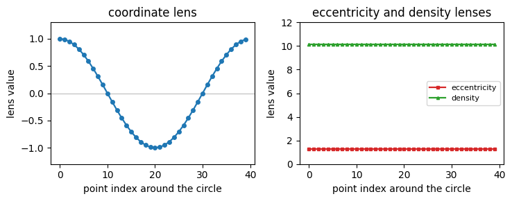
Fig. 3. The lens value at each point around the circle. The coordinate lens (left) varies smoothly, while the eccentricity and density lenses (right) stay constant, so only the coordinate lens can be sliced into a meaningful cover.

The figure makes the point at a glance. The coordinate lens traces a smooth wave as you travel around the circle, so its value genuinely changes from point to point. The eccentricity and density lenses stay flat, one constant value for every point. The numbers confirm it. On a forty-point circle the library reports the following ranges.

Lens	Min	Max	Range
Coordinate	-1.0000	1.0000	2.0000
Eccentricity	1.2726	1.2726	0.0000
Density	10.1588	10.1588	0.0000

The coordinate lens spans a range of two. The two intrinsic lenses have a range of zero to four decimal places. On this shape they are blind. The coordinate lens breaks the symmetry by preferring one axis, and it is the lens that recovers the ring. The lesson is not that one lens is better than another. It is that the lens must match the symmetry of the data, and a good default for symmetric geometry is a coordinate projection.

On a real market cloud the situation is usually reversed. A price embedding is rarely symmetric, so the intrinsic lenses carry real information. The eccentricity lens separates the calm center of a range from the extremes of a trend leg. The density lens picks out the levels where price lingered. The coordinate lens is still available when you want to look along a specific axis of the embedding, such as the most recent return. There is no single correct lens. There is only the one that answers the question you are asking of the cloud.

Implementation: CTDAMapperFilter

The lens class is small. It stores one value per point and the range those values span. The enumeration names the three forms, and the class banner records what each form measures.

//+------------------------------------------------------------------+
//| Lens forms available to the Mapper filter                        |
//|                                                                  |
//|  ECCENTRICITY : mean distance to all points (peripheral = high)  |
//|  DENSITY      : Gaussian kernel density estimate (dense = high)  |
//|  COORDINATE   : one embedding coordinate (breaks symmetry)       |
//+------------------------------------------------------------------+
enum ENUM_TDA_FILTER
  {
   TDA_FILTER_ECCENTRICITY = 0,
   TDA_FILTER_DENSITY      = 1,
   TDA_FILTER_COORDINATE   = 2
  };

//+------------------------------------------------------------------+
//| CTDAMapperFilter - the Mapper lens function                      |
//|                                                                  |
//|  Build stores one scalar f[i] per point plus the range           |
//|  [min, max] the cover will later partition.                      |
//+------------------------------------------------------------------+
class CTDAMapperFilter
  {
private:
   double            m_f[];        // filter value per point [N]
   int               m_N;          // number of points
   double            m_min;        // min filter value
   double            m_max;        // max filter value
   ENUM_TDA_FILTER   m_type;       // lens form used
   int               m_coord;      // coordinate index for COORDINATE lens

public:
                     CTDAMapperFilter();
                    ~CTDAMapperFilter() {}

   //--- coordinate to project onto for TDA_FILTER_COORDINATE
   void              SetCoordinate(int c) { m_coord = c; }

   //--- build the lens (distance matrix for ecc/density, cloud for coord)
   bool              Build(const CTDADistance   &dist,
                           const CTDAPointCloud &cloud,
                           ENUM_TDA_FILTER type = TDA_FILTER_ECCENTRICITY,
                           double densitySigmaFrac = 0.3);

   //--- accessors
   int               Size()  const { return m_N; }
   double            Get(int i) const;
   double            Min()   const { return m_min; }
   double            Max()   const { return m_max; }
   double            Range() const { return m_max - m_min; }
   ENUM_TDA_FILTER   Type()  const { return m_type; }
  };

The class takes both a distance matrix and a point cloud in Build. The eccentricity and density lenses need the distances. The coordinate lens needs the cloud itself. Passing both keeps a single entry point for all three forms. The densitySigmaFrac argument sets the width of the Gaussian used by the density lens, as a fraction of the largest pairwise distance.

The Build method is one switch over the three forms, followed by a pass that records the range.

//+------------------------------------------------------------------+
//| Build the lens values and their range                            |
//+------------------------------------------------------------------+
bool CTDAMapperFilter::Build(const CTDADistance   &dist,
                             const CTDAPointCloud &cloud,
                             ENUM_TDA_FILTER type,
                             double densitySigmaFrac)
  {
   m_N    = dist.Size();
   m_type = type;
   if(m_N < 2)
     {
      Print("TDAMapperFilter::Build - need at least 2 points");
      return false;
     }

   ArrayResize(m_f, m_N);

   if(type == TDA_FILTER_COORDINATE)
     {
      //--- project onto a single embedding coordinate
      int c = m_coord;
      if(c < 0 || c >= cloud.Dim())
        {
         Print("TDAMapperFilter::Build - coordinate out of range");
         return false;
        }
      for(int i = 0; i < m_N; i++)
         m_f[i] = cloud.GetCoord(i, c);
     }
   else if(type == TDA_FILTER_DENSITY)
     {
      //--- Gaussian kernel density: sum_j exp(-d^2 / (2 sigma^2))
      double sigma = densitySigmaFrac * dist.MaxDistance();
      if(sigma <= 0.0) sigma = 1.0;
      double inv2s2 = 1.0 / (2.0 * sigma * sigma);
      for(int i = 0; i < m_N; i++)
        {
         double s = 0.0;
         for(int j = 0; j < m_N; j++)
           {
            double d = dist.Get(i, j);
            s += MathExp(-d * d * inv2s2);
           }
         m_f[i] = s;
        }
     }
   else
     {
      //--- eccentricity: mean distance to all points, sum_j d(i,j) / N
      for(int i = 0; i < m_N; i++)
        {
         double s = 0.0;
         for(int j = 0; j < m_N; j++)
            s += dist.Get(i, j);
         m_f[i] = s / m_N;
        }
     }

   //--- record range
   m_min = m_f[0];
   m_max = m_f[0];
   for(int i = 1; i < m_N; i++)
     {
      if(m_f[i] < m_min) m_min = m_f[i];
      if(m_f[i] > m_max) m_max = m_f[i];
     }
   return true;
  }

The coordinate branch is a single read per point. The density branch is a double loop, order N squared, because each point sums a weight against every other. The eccentricity branch is the same double loop with a plain sum instead of a Gaussian. The final loop records the minimum and maximum, which is all the cover needs to lay out its intervals.

Notice that the two intrinsic lenses cost order N squared, but the distance matrix they read has already been computed once. The lens does not recompute distances. It reads them. For the cloud sizes a Mapper graph is built from, a few hundred points, this cost is negligible.

The reader accessors are trivial by comparison. Get returns one lens value with a bounds check, and Min, Max and Range expose the span the cover will partition.

//+------------------------------------------------------------------+
//| Bounds-checked lens value access                                 |
//+------------------------------------------------------------------+
double CTDAMapperFilter::Get(int i) const
  {
   if(i < 0 || i >= m_N) return 0.0;
   return m_f[i];
  }

A missing index returns zero rather than reading out of bounds. This defensive default runs through the whole library. No accessor is allowed to fault on a bad index.

The Cover: Overlapping Intervals

The cover slices the range of the lens into intervals. Two parameters control it. The resolution is the number of intervals. The gain is how much each interval overlaps its neighbors, given as a fraction between zero and one.

The intervals are laid out evenly. Let the lens range be from min to max. The library defines a step, a center for each interval, and a half-width.

step = (max - min) / resolution

center(k) = min + (k + 0.5) * step

half = 0.5 * step * (1 + gain)

Interval k then runs from center(k) minus half to center(k) plus half, and a point belongs to it when its lens value falls inside that range, endpoints included. When the gain is zero, the half-width is exactly half a step, and the intervals tile the range edge to edge with no overlap. When the gain is positive, each interval grows past its neighbors, and points in the overlap region belong to two intervals at once.

That overlap is essential. If a point lands in two intervals, it will later belong to a node in each interval, creating a shared point between the nodes. Shared points become graph edges. Without overlap there are no shared points, and the graph falls apart into disconnected pieces. The gain is the dial that controls how strongly the graph holds together. We build the nodes and edges in the next article, but the reason the cover overlaps at all is worth stating now.

To make the layout concrete, take the coordinate lens on the circle, whose range is -1 to 1. With resolution 6, the step is 2 / 6 = 0.3333. With gain 0.3, the half-width is 0.5 * 0.3333 * 1.3 = 0.2167. The first interval is centered at -0.8333 and runs from -1.05 to -0.6167. The second is centered at -0.5 and runs from -0.7167 to -0.2833. The two intervals overlap between -0.7167 and -0.6167. A point whose lens value lands in that strip belongs to both.

The endpoints are included on both sides of each interval on purpose. A point whose lens value lands exactly on a boundary must belong to that interval, not fall through a gap between two of them. With the gain at zero this matters at the seams where the intervals touch. With a positive gain the overlap already covers the seams, and the inclusive test simply keeps the membership unambiguous.

The two parameters pull in different directions, and it is worth knowing which does what before tuning them.

Parameter	Effect of raising it	Typical range
resolution	More intervals, a finer graph with more nodes and more detail	5 to 15
gain	More overlap, more shared points, a better connected graph	0.2 to 0.5

Raising the resolution too far splits the cloud into intervals so thin that each holds only a handful of points, and the graph fragments. Raising the gain too far merges everything into one blob. The defaults used throughout this article, a resolution of six and a gain of 0.3, sit in the middle of both ranges. On the forty-point circle they produce the following cover.

Interval	Low	High	Center	Members
0	-1.0500	-0.6167	-0.8333	11
1	-0.7167	-0.2833	-0.5000	8
2	-0.3833	0.0500	-0.1667	6
3	-0.0500	0.3833	0.1667	6
4	0.2833	0.7167	0.5000	8
5	0.6167	1.0500	0.8333	11

The member counts are symmetric, 11, 8, 6, 6, 8, 11. The two end intervals hold more points than the middle ones. This is the circle showing through the lens. Near the turning points of the coordinate axis the ring doubles back on itself, so more points share a similar coordinate value there. The counts sum to more than forty because the overlap regions are counted twice, once for each interval that claims them. That double counting is exactly the shared membership the graph will later turn into edges.

Implementation: CTDAMapperCover

The cover stores its geometry and a list of which points fall in each interval. The membership is kept in a compressed layout: one flat array holds every point index for every interval, back to back, and an offset array marks where each interval's block begins. This is the same idea as a compressed sparse row, and it avoids allocating a separate array per interval. The class banner records the interval formula alongside the members.

//+------------------------------------------------------------------+
//| CTDAMapperCover - splits the lens range into overlapping bins    |
//|                                                                  |
//|  resolution : number of intervals                                |
//|  gain       : overlap fraction in [0,1)                          |
//|                                                                  |
//|  Interval k (k = 0 .. resolution-1):                             |
//|     step   = (max - min) / resolution                            |
//|     center = min + (k + 0.5) * step                              |
//|     half   = 0.5 * step * (1 + gain)                             |
//|     bin_k  = [center - half, center + half]  (inclusive)         |
//|                                                                  |
//|  gain = 0 makes the bins tile the range with touching edges;     |
//|  gain > 0 makes adjacent bins overlap, which is what links the   |
//|  Mapper graph.                                                   |
//|                                                                  |
//|  Membership is stored CSR-style: m_members holds every           |
//|  (interval, point) pair contiguously, m_offset[k] marks where    |
//|  interval k begins.                                              |
//+------------------------------------------------------------------+
class CTDAMapperCover
  {
private:
   int               m_resolution;    // number of intervals
   double            m_gain;          // overlap fraction
   double            m_min;           // lens range low
   double            m_max;           // lens range high
   double            m_step;          // (max-min)/resolution
   double            m_half;          // half-width of each interval
   int               m_N;             // number of points

   int               m_members[];     // flattened member point indices
   int               m_offset[];      // [resolution+1] CSR offsets

public:
                     CTDAMapperCover();
                    ~CTDAMapperCover() {}

   //--- build the cover from a lens
   bool              Build(const CTDAMapperFilter &filter,
                           int resolution, double gain);

   //--- geometry queries
   int               Resolution()   const { return m_resolution; }
   double            IntervalCenter(int k) const;
   double            IntervalLo(int k)     const;
   double            IntervalHi(int k)     const;

   //--- membership
   int               MemberCount(int k) const;
   int               GetMembers(int k, int &out[]) const;
  };

The Build method fills that layout in two passes. Before either one, it validates its inputs and handles the case where the lens is constant.

//+------------------------------------------------------------------+
//| Build overlapping intervals and CSR membership                   |
//+------------------------------------------------------------------+
bool CTDAMapperCover::Build(const CTDAMapperFilter &filter,
                            int resolution, double gain)
  {
   m_N = filter.Size();
   if(m_N < 1)
     {
      Print("TDAMapperCover::Build - empty lens");
      return false;
     }
   if(resolution < 1)
     {
      Print("TDAMapperCover::Build - resolution must be >= 1");
      return false;
     }
   if(gain < 0.0 || gain >= 1.0)
     {
      Print("TDAMapperCover::Build - gain must be in [0,1)");
      return false;
     }

   m_min  = filter.Min();
   m_max  = filter.Max();
   m_gain = gain;

   double range = m_max - m_min;

   //--- degenerate lens (all values equal): one interval holds all points
   if(range <= 1e-12)
     {
      m_resolution = 1;
      m_step = 0.0;
      m_half = 0.0;
      ArrayResize(m_offset, 2);
      ArrayResize(m_members, m_N);
      m_offset[0] = 0;
      m_offset[1] = m_N;
      for(int i = 0; i < m_N; i++) m_members[i] = i;
      return true;
     }

The degenerate branch is the circle problem from the lens section, handled cleanly. If the eccentricity or density lens returns one constant value, the range is zero, and there is nothing to slice. Rather than divide by that range and produce garbage, the cover collapses to a single interval that holds every point. The graph built from it will be a single node. That is the honest answer. A lens that cannot distinguish the points cannot reveal any structure.

When the range is positive, the two passes run. The first pass counts how many points fall in each interval. A prefix sum turns those counts into offsets. The second pass walks the points again and drops each one into its interval's block.

   m_resolution = resolution;
   m_step = range / resolution;
   m_half = 0.5 * m_step * (1.0 + gain);

   //--- pass 1: count members per interval
   ArrayResize(m_offset, m_resolution + 1);
   ArrayInitialize(m_offset, 0);

   for(int i = 0; i < m_N; i++)
     {
      double fi = filter.Get(i);
      for(int k = 0; k < m_resolution; k++)
        {
         double c = m_min + (k + 0.5) * m_step;
         if(fi >= c - m_half && fi <= c + m_half)
            m_offset[k + 1]++;
        }
     }

   //--- prefix sum -> CSR offsets
   for(int k = 0; k < m_resolution; k++)
      m_offset[k + 1] += m_offset[k];

   int total = m_offset[m_resolution];
   ArrayResize(m_members, (total > 0 ? total : 1));

   //--- pass 2: fill members using a moving cursor per interval
   int cursor[];
   ArrayResize(cursor, m_resolution);
   for(int k = 0; k < m_resolution; k++)
      cursor[k] = m_offset[k];

   for(int i = 0; i < m_N; i++)
     {
      double fi = filter.Get(i);
      for(int k = 0; k < m_resolution; k++)
        {
         double c = m_min + (k + 0.5) * m_step;
         if(fi >= c - m_half && fi <= c + m_half)
           {
            m_members[cursor[k]] = i;
            cursor[k]++;
           }
        }
     }
   return true;
  }

The first pass writes its counts one slot to the right, into m_offset[k + 1]. The prefix sum then converts those counts in place into starting offsets. After the sum, m_offset[k] is the index where interval k begins, and m_offset[k + 1] is where it ends. The second pass keeps a cursor per interval, starting at each interval's offset, and advances it as it writes each member. The membership test is identical in both passes, so a point counted in the first pass is guaranteed a slot in the second.

Two passes cost twice the work of one, but they buy a single contiguous allocation for all membership. The alternative, growing a separate list per interval, would allocate many small arrays and resize them repeatedly. For a structure that a sliding indicator will rebuild on every step, the flat layout is the right call.

The accessors read that layout back. MemberCount is a subtraction of two offsets. GetMembers copies one interval's slice into a caller array.

//+------------------------------------------------------------------+
//| Number of points falling in interval k                           |
//+------------------------------------------------------------------+
int CTDAMapperCover::MemberCount(int k) const
  {
   if(k < 0 || k >= m_resolution) return 0;
   return m_offset[k + 1] - m_offset[k];
  }

//+------------------------------------------------------------------+
//| Copy the member point indices of interval k into out[]           |
//+------------------------------------------------------------------+
int CTDAMapperCover::GetMembers(int k, int &out[]) const
  {
   if(k < 0 || k >= m_resolution)
     {
      ArrayResize(out, 0);
      return 0;
     }
   int lo = m_offset[k];
   int hi = m_offset[k + 1];
   int cnt = hi - lo;
   ArrayResize(out, (cnt > 0 ? cnt : 0));
   for(int t = 0; t < cnt; t++)
      out[t] = m_members[lo + t];
   return cnt;
  }

These two are the interface the clustering step will use in the next article. It asks the cover for the members of each interval, one interval at a time, and clusters them. Everything in this article exists to answer that one query correctly.

The Demo Script

The script TDA_Mapper_Demo.mq5 ties the two classes together. It builds a cosine series whose two-dimensional delay embedding is a circle, computes all three lenses on that cloud, and builds the cover of the coordinate lens. The core of the script is short.

   //--- 2. three lens forms on the SAME cloud
   CTDAMapperFilter fCoord, fEcc, fDens;
   fCoord.SetCoordinate(0);
   fCoord.Build(dist, cloud, TDA_FILTER_COORDINATE);
   fEcc.Build(dist, cloud, TDA_FILTER_ECCENTRICITY);
   fDens.Build(dist, cloud, TDA_FILTER_DENSITY, 0.3);

   ReportLens("coordinate", fCoord);
   ReportLens("eccentricity", fEcc);   // near-constant on a circle: motivates coord lens
   ReportLens("density", fDens);

   //--- 3. cover of the coordinate lens
   CTDAMapperCover cover;
   if(!cover.Build(fCoord, InpRes, InpGain)) { Print("cover build failed"); return; }

Run the script on any chart and it reports the two tables shown earlier: the three lens ranges, and the six cover intervals with their member counts. The coordinate lens spans two, the eccentricity and density lenses are flat, and the intervals carry the symmetric 11, 8, 6, 6, 8, 11 membership. The image below shows the Experts log from a run.

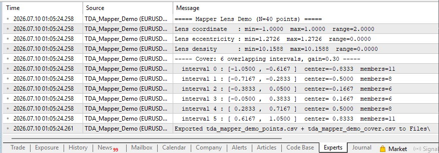
Fig. 4. The Experts log of the demo: the three lens ranges and the six cover intervals with their member counts.

The cosine series is chosen so the embedding is an exact circle, which makes the output easy to check by eye and by number. Feed the same script a window of real closes instead, and the cloud loses its symmetry. The coordinate lens still spans a real range, and now the eccentricity and density lenses do too. The cover table then reflects where the price cloud is dense and where it is sparse, rather than the tidy symmetry of a circle.

The script also exports one file with a lens value per point and one with the interval bands. Those two files produced the colored cloud figure at the top of this article. Nothing here yet forms a node or an edge. The cloud has simply been reduced to a value per point and a set of overlapping bins.

What's Next

We have a lens and a cover. We do not yet have a graph. The next article builds the two steps that produce it.

• Clustering the points inside each interval into nodes, using single linkage on the distance matrix.
• Joining nodes that share points into edges, which is where the overlap in the cover finally pays off.
• The circle, run end to end, will come out as a ring of nodes, the shape we have been aiming at from the start.

Conclusion

What you have at the end of this article is a reproducible foundation for the Mapper graph, and the means to confirm it is correct before building anything on top of it. You can take a price cloud, reduce it to one value per point with a lens of your choice, and slice the range of those values into an overlapping cover. You can run the demo, read the lens ranges and the interval table it prints, and reproduce the member counts exactly.

CTDAMapperFilter produces one scalar f[i] per point and reports the minimum, maximum, and range for the chosen lens form, whether eccentricity, density, or coordinate projection. That range is your degeneracy test: if it comes out zero, the intrinsic lenses are blind on symmetric data, and the cover is right to collapse to a single interval. CTDAMapperCover takes that lens, a resolution, and a gain, and builds the overlapping intervals, storing membership in a flat layout of one contiguous index array plus an offset per interval. The demo prints both the lens ranges and a table of intervals, their low, high, center, and member counts, so you can check the cover by eye and by number.

Three checks confirm the artifacts before you move on.

• The lens range should be non-zero wherever you expect structure. If it is zero, either switch to the coordinate lens or re-embed the data.
• The member counts should track the density of the cloud, and when the gain is positive, the members summed across all intervals should exceed N, since each overlap point is counted twice.
• Start from a resolution near 5 to 15 and a gain near 0.2 to 0.5, then tune from there.

With these two blocks built and validated, you are ready for the next article. It clusters the points inside each interval into nodes, using single linkage on the distance matrix, then joins nodes that share points into edges. Run end to end, the circle of this article comes out as a ring of nodes, the compact Mapper graph that motivated the whole exercise.

• CTDAMapperFilter assigns one value to every point, by eccentricity, density, or coordinate projection, and reports the range those values span.
• CTDAMapperCover slices that range into overlapping intervals and records which point indices fall in each.

#	Filename	Type	Description
1	TDAMapperFilter.mqh	Header	Mapper lens function (this article)
2	TDAMapperCover.mqh	Header	Overlapping-interval cover (this article)
3	TDAPointCloud.mqh	Header	Takens phase-space embedding (reused, needed by the lens)
4	TDADistance.mqh	Header	Pairwise distance matrix (reused, needed by the lens)
5	TDA_Mapper_Demo.mq5	Script	Lens and cover demonstration (this article)