Defining your Edge (Part 2): Using Divergence Mapping and a Temporal Fusion Transformer in a Trading Robot

Introduction

A central and common challenge in technical analysis does not stem from spotting trends, but in surviving the transitional spaces between them. How can false breakouts be avoided? To navigate these, we argue here that one needs to look beneath the surface and focus on the subtle and concealed changes in velocity before structural changes unfold. By pairing Divergence Mapping with a Temporal Fusion Transformer attention layer, we aim to create a solid alternative forecasting metric.

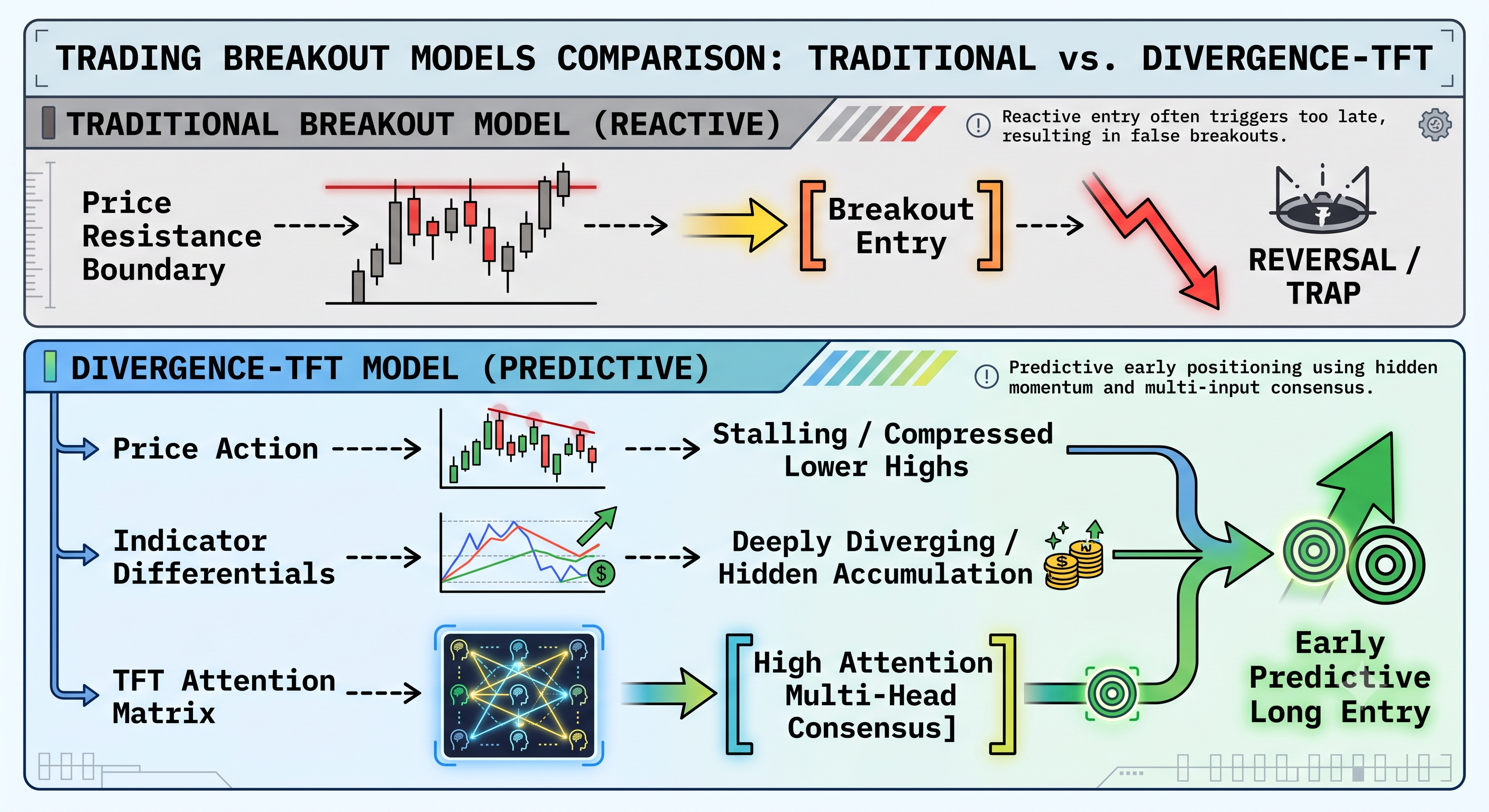
This particular combo of slope calculus and non-linear sequential weighting may not be widely in use. Careful testing and parameter tuning is bound to be a prerequisite for many tradable assets on offer. This article only acts as a foundational step in better understanding and merging these two engines when developing trade entry signals. Our final output is a Trade Robot. In my opinion (not an official MetaQuotes statement), that Expert Advisors with their induction in MQL5, about '09 were meant to be strict positional traders, and not capable of executing concurrent buy and sell orders. 

IMO the "Advisor" tag was attributed because these experts output probability distributions of the market outlook and are not tied per se to the actual trading operations. A Trade Robot on the other hand, though also capable of using probability distributions, is not coded with MQL5 CExpertSignal class and can have a more customized order flow that departs from MQL5's position-based flow. We have moved on in accepting diverse trade approaches to the market, since '09, whereby even though there are many are positional traders today, we still have hedging based traders. With this extra flexibility, this Trading Robot from this article, when merged with what we had in the last article and hopefully more to come, could give us a repository. This "store" would allow one to fine-tune their trading edge while freeing them from a risky overreliance on highly correlated mainstream indicators and systems.

Divergence-TFT Paradigm

The paradigm of Divergence Mapping and TFT is able to overcome delays of trap-prone signals that stem from lagging indicators by rejecting single-point breakout confirmation. This pairing uses two core pillars: a Velocity Differential engine that tracks rate changes between price and momentum; and a time-based attention-layer of a neural network that evaluates their sequence. When we feed hidden structural discrepancies into a Temporal Fusion Transformer, it sieves out the noise and secures the predictive edge. This allows more precise positioning prior to a breakout.

Suited Markets and Niches

The Divergence-TFT paradigm is clearly built to address structural failures that can show up in specific trading profiles and macroeconomic settings. In modern electronic markets, a major weakness for quantitative systems is their reliance on overly correlated indicators. When an entire trading desk or algorithmic suite uses derivative mathematical models that are structurally dependent on identical primitives - like moving averages, variance, or common volatility bands - their execution points will tend to cluster. This overlapping can create acute liquidity pools that larger institutional market-making algorithms can actively target. This in turn increases stop-hunting behaviors that are often characterized by false breakout loops, which can disrupt conventional trend-following systems.

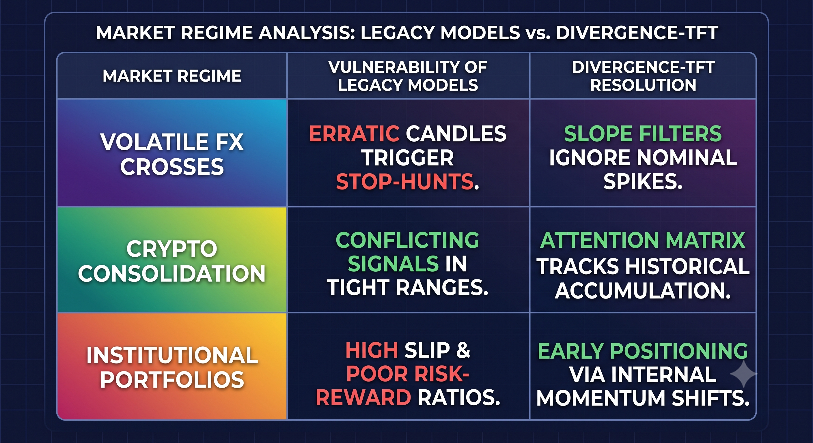
This Divergence-TFT paradigm could be used as a means of guarding systems from clustered execution points where institutional stop-hunting runs amok. This dual engine mode, in this setting, is therefore meant to serve three separate market niches: filtering out volatile candles e.g. with FX crosses; tracking hidden historical accumulation e.g. in crypto consolidation; improving risk reward ratios by earlier position entry in non-correlated momentum tracking.

The Synergy

Automated trading systems can suffer from one-engine vulnerabilities: rigid lagging indicators akin to a car driver who only looks at his rear view mirror, or unguided deep learning networks that overfit a particular market static like night-vision goggles that amplify visual noise amplification.

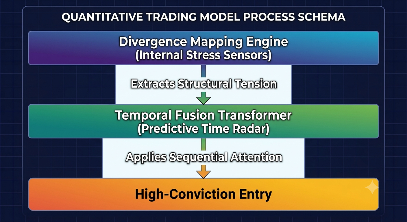
This two-engine paradigm tries to resolve this via a balanced pipeline. The Divergence Mapping engine serves as car-suspension sensors, constantly getting structural tension by measuring weight and torque differentials between price and indicator slopes. This clean data passes to a proxy Temporal Fusion Transformer that is a forecasting radar. It uses sequential multi-head attention profiles over time horizons, filtering noise for high-conviction entries.

Math Definitions

In order to construct a rigorous proofing framework, it could be informative to lay out the formulae that govern both the structural divergence engine and the sequential attention processing layer. 

The Algorithm

This engine does not view raw indicators as absolute boundaries. Rather, it measures the slope differential between asset changes in price and indicator vectors over a preset lookback window, N. If we let P stand for the price series vector (such as bar close prices) and I represent the indicator vector values (such as raw DeMarker or RSI readings); then first of all the raw momentum slope for both price and the indicator is calculated as a simple finite change over the lookback window N:

where:

• Vector_0 (e.g. P_0, I_0) is the current value of the respective vector (P or I).
• Vector_N-1} (e.g. P_N-1, I_N-1) is the historical value of that same vector at the set window start.
• N is the number of temporal periods (bars) limiting the lookback window.

Given that price scales can vary a lot depending on the asset under consideration (e.g. fractional pips are common in forex yet thousands of dollars get applied in Bitcoin), the raw price slope needs to be normalized relative to its baseline value in order to make it mathematically comparable to bounded oscillators. The normalized price slope follows the formula:

Where:

• NormSlope_P is the sought normalized slope of the price series P.
• Slope_P is the raw momentum slope of the price series, as defined in previous equations.
• P_N-1 is the historical price at the very start of the lookback period, serving as our base valuation for this normalization.

The hidden shift in momentum or divergence differences (Delta_div) can then be isolated by getting the direct variance between these two normalized trajectories:

A structural signal is thus confirmed if this divergence value is more than a predefined sensitivity parameter:

The Network

If we had a full-scale deep-learning production environment, then the Temporal Fusion Transformer would use multi-head attention mechanisms that are merged with variable selection networks in order to dynamically determine weight sequence importance. In this native MQL5 proxy architecture, we simply simulate this sequence's contextualization by mapping inputs into separate time based states. These are t_1, t_2, and t_3. Then we execute an attention gating. If we let the network inputs be mapped as vector parts that stand for separate time horizons, then:

• t_1 would be the immediate or current temporal state mapping high-frequency velocity
• t_2 would be the preceding temporal state that maps to our mid-frequency anchor
• t_3 is then the macro sequential momentum block mapping to a low-frequency context

The multi-head attention weights are clearly given fixed priorities with a bias towards recent market behavior while also preserving some historical relevance:

Where:

• W is the static multi-head attention weight vector meant for sequence priority over separate temporal horizons.
• q k_v_weight1 (0.55) is the attention weight given to the recent temporal state (t_1). This gives a heavy recency bias for the real-time market vector.
• q k_v_weight2 (0.30) is our attention weight assigned to the prior state (t_2), acting as the mid-frequency sequential anchor.
• q k_v_weight3 (0.15) is the weight given to the furthest momentum block (t_3), that gives broad historical context to the network.

The composite attention scores for the buy matrix (alpha_buy) and the sell matrix (alpha_sell) are worked out by taking the inputs through an activation simulation  function that sets apart positive and negative momentum components:

Where:

• alpha_buy is the composite attention score for the buy matrix, adding up plus momentum parts.
• alpha_sell is our overall attention score for the sell, aggregating the magnitude of negative momentum parts.
• n stands for the index of the specific time period being processed (n = 1 for t_1, n = 2 for t_2, n = 3 for t_3).
• t_n is the incoming divergence signal for the n-th state.
• max(0, t_n) is an activation filter for isolating only positive (bullish) values. This reduces negative inputs to zero.
• |min(0, t_n)| is the activation filter that isolates only negative (bearish) values and brings back their absolute magnitude.
• W_n is the corresponding fixed multi-head attention weight assigned to the n-th state from the priority vector W.

The final decision boundary ensures a very strict mutual exclusivity constraint. This means a structural attention breakout fires only when one attention track goes past the threshold parameter while the opposing direction remains subcritical:

MQL5 Implementation

Connecting abstract Math and a working executable model necessitates translation to code. In this section, we systematically try to deconstruct the MQL5 implementation of the divergence-TFT paradigm. Every function, variable array, as well as logical boundary is explicitly designed to keep the integrity and model's edge as covered above. We also try to be lean on memory use when executing.

Indicator Choice Rationale

With the plethora of technical indicators on offer, why did we pick the pair Welles' RSI and the DeMarker? Our choice is always hinted with subjectivity, and the Divergence framework depends on separating structural anomalies between price and momentum. Nonetheless, not all momentum indicators are the same. The reason we pair the DeMarker to the Relative Strength Index (RSI) is fairly deliberate and based on the "orthogonal dimensions"| of market velocity.

F. Welles Wilder's Relative Strength Index is a raw measure of price velocity size. It compares the mean of successive closing price gains to the mean closing price losses, over a set time window.  Since this RSI is fairly rooted in closing price values, it also serves as a proxy for consensus valuation at the end of a time period. It keeps tabs on the overall velocity of the trend.

Conversely, Thomas DeMark's indicator works on a separate premise. This indicator focuses a lot on intra-period extremes while putting emphasis on the relationship between current high/low and the prior high/low. It tries to get a sense of buying/selling pressure by putting a metric to how deeply the current bar exceeds the structural extremes of the prior bar. Given that it does not depend a lot on the final closing price, the DeMarker acts as a highly sensitive proxy to intraday price tension and exhaustion.

Uniting these two indicators, our algorithmic engine gets fed a three dimensional view of the market. The RSI gives the macro-velocity (speed of closing consensus) while the DeMarker gets us the micro-exhaustion or the fading of extreme pressures. When these two decoupled indicators concurrently diverge from the underlying slope of price, the statistical likelihood of a false signal being in play diminishes significantly. In essence we would no longer be observing a quirk in the closing prices but rather we would be looking at deceleration in market-price and this backdrop is ideal for our Divergence Mapping.

Divergence Mapping Algorithm

Our starting component of this model is the engine in charge of getting the hidden changes in momentum from market-price. This is handled by the 'CalculateDivergenceShift' method. This function takes raw scale variant market data and changes it into a normalized differential capable of being evaluated regardless of the asset being traded.

//+------------------------------------------------------------------+
//| Mathematical Engine: Divergence Mapping (Slope Differential)     |
//+------------------------------------------------------------------+
double CalculateDivergenceShift(double &priceData[], double &indicatorData[])
  {
   int N = ArraySize(priceData);
   if(N < 2)
      return 0.0;

This function takes in two dynamic arrays: 'priceData' and 'indicatorData'. Importantly, these arrays get passed as a reference via the operator '&' marking them as objects, with a memory address. In low-timeframe systematic trading, passing large historical data arrays can create large memory overhead as well as compute lag. Since the entire array would be duplicated in memory with every function call. Passing it as a reference enables the algorithm to directly access memory addresses  of the arrays, and this in turn enables microsecond execution times, and this is important when processing rapid tick/price-bar data. The integer N stands for our dynamic lookback window. The initial boundary check 'if(N < 2)' serves as a safety check; when computing the slope a minimum of two coordinate points in time are prerequisite. If the buffer does not populate, the function would safely abort by returning a neutral zero.

//--- Calculate slope (momentum) of Price vs Indicator
   double priceSlope = (priceData[0] - priceData[N - 1]) / N;
   double indSlope = (indicatorData[0] - indicatorData[N - 1]) / N;

In the listing above, the engine works out the linear approximation of the vectors. The most recent data point is always kept at index 0 however the oldest data in the window is assigned at 'N-1'. By subtracting the historical border from the current border and diving by the time distance 'N', we derive the raw slope. This gives us the absolute rate of change. However, a critical math conflict can arise here: the 'indSlope' value is bounded by the oscillator's limits and this can be either [0, 100] or [0.0, 1.0]. On the other hand though, the 'priceSlope' is completely unbothered by such constraints with its value depending on the asset being traded. A slope calculation on a volatilie asset like BTC can give us a raw value in the hundreds while a similar calculation on the pair GBPUSD could give us something close to 0.00001.

//--- Normalize Price Slope to match generic indicator scale roughly
   double normPriceSlope = priceSlope / priceData[N - 1];

To help resolve this dimensional conflict, the 'priceSlope' needs to be aggressively normalized. If we divide the raw price by its historical boundary price at the index N-1, we would be able to convert the absolute price change into a standardized percentage-based differential. Our approach removes the asset's nominal value, and leaves us a pure representation of geometric velocity. This normalized slope is now "dimensionally compatible" with the indicator slope we referenced earlier.

//--- Differential represents the divergence (Hidden Momentum Shift)
   double divergenceShift = indSlope - normPriceSlope;
   return divergenceShift;
  }

The last calculation in this function, in many ways, represents the core edge of our engine. Since we subtract the normalized price velocity from the indicator velocity, we are able to separate the Delta_div parameter. When price is falling steeply (a negative normalized slope) and yet the indicator's slope is on the up, this equation would give us a huge positive divergence shift. This isolated integer is the pure math expression of a hidden structural anomaly. It is filtered of surface-level chart noise.

TFT Proxy Network

Having identified price-structural anomalies, we now move on to giving the raw price feed some context. In large deep-learning networks, a Temporal Fusion Transformer uses the selection of variables and multi-head attention on large sequences of data. We want to replicate part of this in a native lightweight MQL5 setting that does not necessitate external Python integration. The 'EvaluateTFTNetwork' function would act as a precision proxy that uses simulated attention weights.

//+------------------------------------------------------------------+
//| AI Engine: Temporal Fusion Transformer Proxy (Attention Network) |
//+------------------------------------------------------------------+
int EvaluateTFTNetwork(double t1_signal, double t2_signal, double t3_signal)
  {
//--- Simulating multi-head attention weights based on sequence importance
   double q_k_v_weight1 = 0.55; // Most recent temporal priority
   double q_k_v_weight2 = 0.30; // Mid temporal priority
   double q_k_v_weight3 = 0.15; // Furthest temporal priority

Our network takes in three separate temporal state inputs: t_1, t_2, and t_3. These are for the recent/immediate velocity, the preceding mid-frequency momentum, and the broad historical context respectively. The weights 'q_k_v_weight' help simulate the dot products of the Query, key, and value matrices that are found in a real transformer block. The distribution of these weights is always asymmetric. A weight of '0.55' is given to the most recent state t_1, and this enforces a strong recency bias. The market's immediate structural tension is often the most probabilistic relevant variable. The weights for decaying of '0.30' and '0.15' for the older states give the network the requisite historical context while a;so not allowing the "stale" data to overpower the real-time stream. 

//--- Contextualizing outputs through a simulated activation
   double attentionBuy  = 0.0;
   double attentionSell = 0.0;
   if(t1_signal > 0)
      attentionBuy += t1_signal * q_k_v_weight1;
   else
      attentionSell += MathAbs(t1_signal) * q_k_v_weight1;
   if(t2_signal > 0)
      attentionBuy += t2_signal * q_k_v_weight2;
   else
      attentionSell += MathAbs(t2_signal) * q_k_v_weight2;
   if(t3_signal > 0)
      attentionBuy += t3_signal * q_k_v_weight3;
   else
      attentionSell += MathAbs(t3_signal) * q_k_v_weight3;

This sequence stands for the proxy activation function and loosely models after the Rectified Linear Unit (ReLU) while maintaining directional bias. The network launches two distinct competing attention matrices: one for longs (buying) accumulation and one for shorts (selling) accumulation. Every temporal signal gets evaluated. When the signal turns out positive, this indicates an underlying bullish divergence. The magnitude of this signal would get multiplied by its respective attention weight and then added to the 'attentionBuy' matrix. When the signal is negative, its magnitude is retrieved via 'MathAbs()', and added to the competing 'attentionSell' matrix. Since we enforce this strict segregation, our network is able to independently track the build-up of bullish pressure across the sequence instead of merely averaging them out which would risk losing information on underlying price action. 

   bool buyBreakout = (attentionBuy >= InpAttentionThresh);
   bool sellBreakout = (attentionSell >= InpAttentionThresh);
   if(buyBreakout && !sellBreakout)
      return 1;
   if(sellBreakout && !buyBreakout)
      return -1;
   return 0;
  }

The concluding section in the above function acts as a decision boundary. The accumulated attention in both matrices is tested against the 'InpAttentionThresh' parameter. A critical fail-safe is implemented here through a mutual exclusivity constraint. For our network to allow a buy signal (by returning 1), the Boolean should be set to 'true', AND the 'sellBreakout' Boolean needs to be assigned 'false'. When we have erratic, very volatile market phases both the buy and sell attention matrices can concurrently spike. This common occurrence especially in major macroeconomic news releases would lead to our network recognizing "structural chaos". This chaos would have both outputs for long and short neutralized and the return value set to zero.

The Operational Modes

To ensure the architecture can be rigorously tested and separated, the running is split into 7 possible use-modes. The chosen mode is controlled by the 'EMode' enumeration which is implemented via a switch statement in the 'OnTick()' loop. 

//+------------------------------------------------------------------+
//| Expert tick function                                             |
//+------------------------------------------------------------------+
void OnTick()
  {
//--- Execute only on a new bar
   datetime timeCurrentBar = iTime(_Symbol, _Period, 0);
   if(timeCurrentBar == timeLastBar)
      
      return;
   int signal = 0; // 0 = No signal, 1 = Buy, -1 = Sell
//--- Route execution to the selected function mode
   switch(InpMode)
     {
      case MODE_DIVERG_PRICE:
         signal = ExecuteDivergencePrice();
         break;
      case MODE_DIVERG_DEMARKER:
         signal = ExecuteDivergenceDeMarker();
         break;
      case MODE_DIVERG_RSI:
         signal = ExecuteDivergenceRSI();
         break;
      case MODE_DIVERG_COMBINED:
         signal = ExecuteDivergenceCombined();
         break;
      case MODE_PRICE_ACTION_TFT:
         signal = ExecutePriceActionTFT();
         break;
      case MODE_INDICATOR_PATTERN:
         signal = ExecuteIndicatorPatternTFT();
         break;
      case MODE_HYBRID_FULL:
         signal = ExecuteHybridFull();
         break;
     }
//--- Process Trading Signals
   if(signal != 0)
     {
      ManagePositions(signal);
      timeLastBar = timeCurrentBar;
     }
  }

Prior to invoking the algorithm or network, the 'OnTick()' function applies a strict time based lock. We compare the time of the current bar to 'timeLastBar', and the Trade Robot guarantees that it only runs the compute intense calculations only once on every new bar open. This can be thought of as a foundational necessity for most robust trading robots. Without this we would find ourselves in a situation where we are evaluating complex divergence mappings on every single incoming tick which would drain a lot of resources not to mention that the "constant repainting" would have new signals flashing and disappearing which give us a very erratic performance. Processing at the bar's open means our model depends only on permanently closed price bars, or immutable historical data. Our model then routes this logic through the seven possible mode options. One of these is the basic divergence mode that is listed as follows: 

//+------------------------------------------------------------------+
//| Signal Generator: Mode 2 (MODE_DIVERG_RSI)                       |
//| Measures momentum divergence between Close price and RSI.        |
//+------------------------------------------------------------------+
int ExecuteDivergenceRSI()
  {
   double rsiVals[], closePrices[];
   ArrayResize(rsiVals, InpLookbackWindow);
   ArrayResize(closePrices, InpLookbackWindow);
   if(CopyBuffer(hRSI, 0, 0, InpLookbackWindow, rsiVals) < InpLookbackWindow)
      return 0;
   if(CopyClose(_Symbol, _Period, 0, InpLookbackWindow, closePrices) < InpLookbackWindow)
      return 0;
   double shift = CalculateDivergenceShift(closePrices, rsiVals);
   if(shift > InpDivergThreshold)
      return 1;
   if(shift < -InpDivergThreshold)
      return -1;
   return 0;
  }

In our mode above, 'ExecuteDivergenceRSI', we start by sizing dynamic arrays to match the selected input lookback window. The 'CopyBuffer' function then safely gets indicator data directly from the system's memory handles while 'CopyClose' secures the price vector. When data fails to copy accurately the function safely aborts. Without an abort, the arrays get fed into the divergence mapping engine with the end shift getting compared against the input threshold. Arguably though, the real power of our model could be demonstrated in mode 7: 

//+------------------------------------------------------------------+
//| Signal Generator: Mode 6 (MODE_HYBRID_FULL)                      |
//| Blends full window divergence outputs across indicators via the  |
//| TFT network or mathematical threshold filtering.                 |
//+------------------------------------------------------------------+
int ExecuteHybridFull()
  {
   double closePrices[], rsiValues[], deMarkerValues[];
   ArrayResize(closePrices, InpLookbackWindow);
   ArrayResize(rsiValues, InpLookbackWindow);
   ArrayResize(deMarkerValues, InpLookbackWindow);
   if(CopyClose(_Symbol, _Period, 0, InpLookbackWindow, closePrices) < InpLookbackWindow)
      return 0;
   if(CopyBuffer(hRSI, 0, 0, InpLookbackWindow, rsiValues) < InpLookbackWindow)
      return 0;
   if(CopyBuffer(hDeMarker, 0, 0, InpLookbackWindow, deMarkerValues) < InpLookbackWindow)
      return 0;
   double pDiverg = CalculateDivergenceShift(closePrices, closePrices); // Price auto-divergence
   double rDiverg = CalculateDivergenceShift(closePrices, rsiValues);
   double dDiverg = CalculateDivergenceShift(closePrices, deMarkerValues);
   if(InpUseTFT)
     {
      //--- Feed mapping into the Neural Net
      return EvaluateTFTNetwork(dDiverg, rDiverg, pDiverg);
     }
   else
     {
      //--- Pure mathematical execution
      if(dDiverg > InpDivergThreshold && rDiverg > InpDivergThreshold)
         return 1;
      if(dDiverg < -InpDivergThreshold && rDiverg < -InpDivergThreshold)
         return -1;
     }
   return 0;
  }

This mode gives us a complete synthesis of the algorithm and network. Rather than feeding raw price data into the neural network, 'ExecuteHybridFull' makes the algorithm act like a deep feature-engineering layer. It works out three separate divergence profiles: an auto-divergence of the price itself, the macro-velocity divergence of the RSI as well as the exhaustion of the DeMarker. These three noise filtered values then get fed as t_1, t_2, and t_3 to the TFT proxy. In essence our network is no longer studying price charts but is scrutinizing attention weights of competing oddities in market price. This then goes on to serve as a verification layer for any breakouts that are forwarded by the divergence mapping algorithm.

Only valid signals then get forwarded to 'ManagePositions()' where order execution is also managed.

Post-Optimization Analysis

We test this model by forward walk following an optimization stint. The forex symbol we use is GBPJPY, and our optimization window is from 2025.01.01 to 2026.01.01. The forward walk test is from 2026.01.01 to 2026.05.01. The key parameters we tuned or optimized were:

• Window size for divergence mapping (InpLookbackWindow)
• Minimum slope differential for valid breakout (InpDivergThreshold)
• Attention threshold for firing signals (InpAttentionThresh)
• Decay weight for sequence historical inputs (InpSeqWeighting)

These were subsequently assigned 44, 0.012, 0.6, and 0.3. The back test report over the optimized period was then as follows:

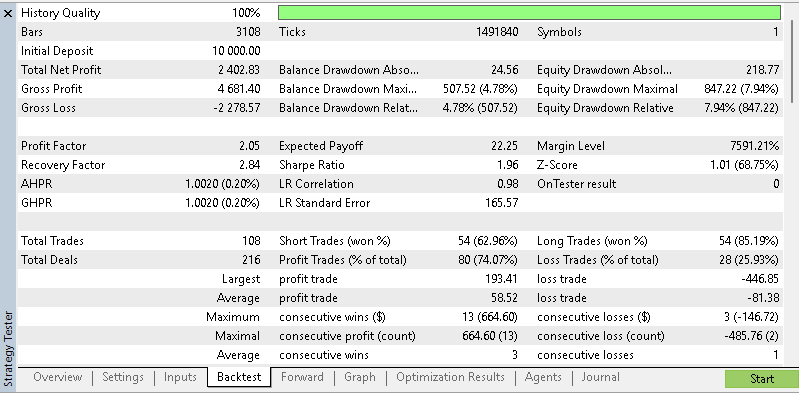
And its following forward walk report for the first four months of 2026 was as follows:

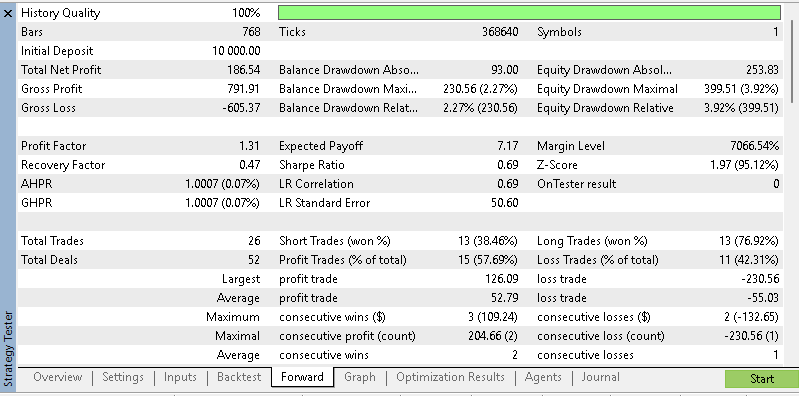
Our testing timeframe is the 2-hour. If we run a test over both the optimized and forward walk periods we are presented with the following equity curve:

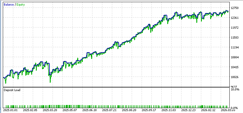
The important forward walk report can be summarized with the 5 key metrics presented in the table below:

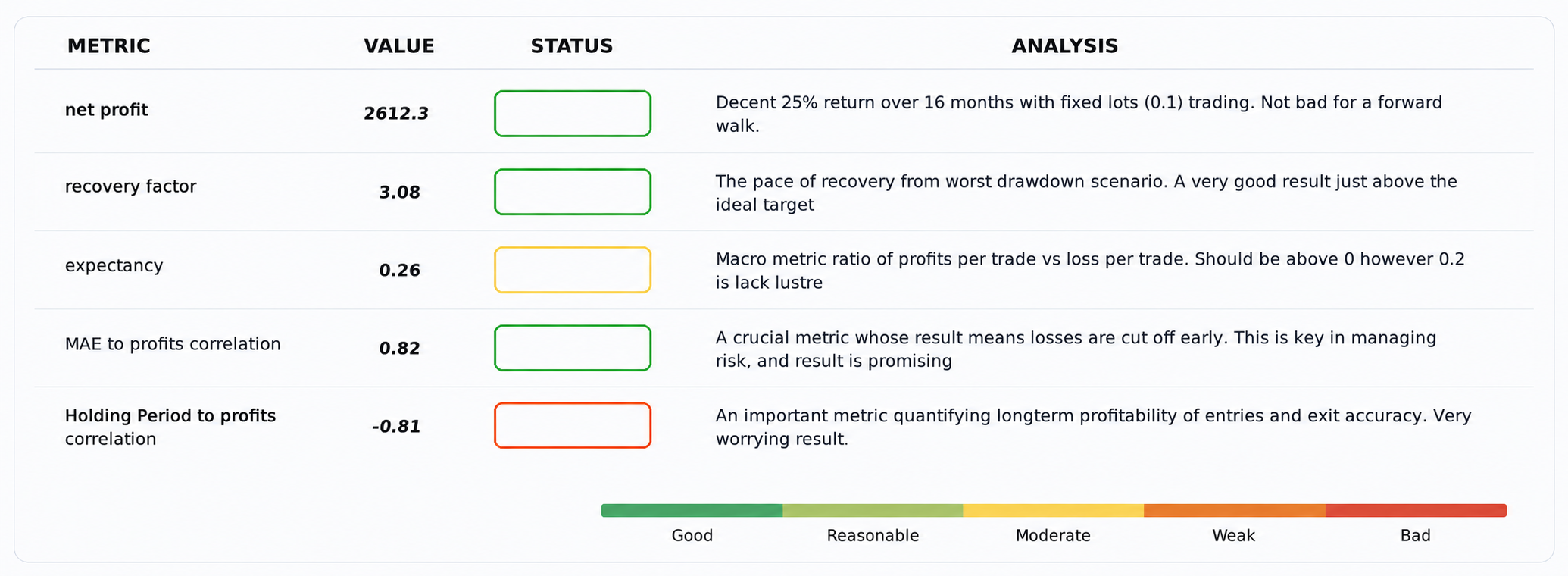
If we dig into these results that span the optimization and forward walk period, we can get a sense of the potential limits of our model when trading the GBPJPY. Over the 268 trades placed our model was able to secure a net profit of $2,625.80 at an overall profit factor of 1.25. One major optimization parameter we tuned, not listed above was whether to use the TFT network or not. Interestingly our best settings opted not to use our TFT, meaning all the extra work we put into this second gate was not utilized! This testing though is for a very small period and on just one symbol therefore as always I will argue that testing on extra symbols and on larger test windows should be done before the baby is thrown out with the bath water.

Conclusion

In summation, the evidence from our 4-month forward walk testing on one forex pair GBPJPY underscores that pairing Divergence Mapping with a Temporal Fusion Transformer proxy gives us a reliable non-correlated trading framework. Instead of acting like a generic predicting tool, this model successfully worked as a surgical filter, spotting underlying accumulation sequences in advance of when they were logged by lagging regular indicators.

Nonetheless, this rigorous multi-period optimization and forward-walk validation on the GBPJPY on the 2-hour timeframe gave us a reality check: the optimal genetic settings did not use the proxy TFT attention network at all. The model solely depended on the raw math divergence engine in order to secure 268 trades for a net profit of $2600, and a drawdown just north of 8%. But rather than discount this network, this finding could stress the point that specialized attention layers need a wider cross-symbol evaluation and longer historical windows in order to avoid instances where the optimization algorithm favors simpler linear structures over sensitive time based matrices. 

Our model could also use some refinement, which is left to the discretion of the reader. Extra refinements that could be adopted are: deep learning integration with python via ONNX where the network we use becomes more comprehensive; and multi-symbol portfolio proofing as suggested already above in order to better test the TFT.

name	description
02 Divergence TFT DeMarker RSI.mq5	Model-Implementing Trade Robot
i.set	Test Optimization Inputs