CSV Data Analysis (Part 7): Statistical Robustness Testing on MQL5 CSV Exports with Monte Carlo Simulation

Introduction

A standard backtest is deterministic: it evaluates a fixed algorithm on a finite historical dataset and produces one performance implementation for a single sequence of market conditions. Determinism ensures repeatability, but it limits retrospective analysis. A single historical run cannot tell whether the result is representative or an outlier among plausible alternatives. For example, a favorable Sortino Ratio may reflect a genuine structural edge, or it may merely be the product of a specific trade sequence that minimized the calculation's downside deviation denominator. Distinguishing between a durable edge and statistical luck requires analytical machinery that evaluates a distribution of potential outcomes rather than a single observed path.

To address this limitation, this article introduces a statistical validation battery consisting of three distinct analytical methods. Permutation testing evaluates whether the observed strategy performance significantly exceeds what chance would produce in the absence of a directional edge. Bootstrap resampling assesses the stability of the performance metrics across alternative, plausible variations of the underlying trade data. Finally, Monte Carlo trade-sequence shuffling randomizes execution order. This shows whether the equity curve and drawdown depend on the historical win/loss sequence or on the trades themselves.

Combined, these three methodologies form a validation framework to evaluate historical performance integrity. The system integrates with the trade-level CSV export pipeline from earlier articles. Developers can run the full battery on any output strategy without changing the Expert Advisor logic.

Note: If you missed Part 6 of this series, you can read it here.

Section 1: Three Statistical Tools and When to Use Each

Permutation Testing

Permutation testing is a non-parametric hypothesis test. It makes no assumptions about the distribution of trade returns and is therefore more appropriate for algorithmic trading data than parametric tests such as the t-test, which assume normality. The test works by computing a test statistic on the observed data, then computing that same statistic on thousands of randomized versions of the data where the effect being tested has been deliberately destroyed. The proportion of randomized results that meet or exceed the observed statistic is the p-value.

A subtle but critical point governs how the randomization must be performed. The Sortino Ratio is order-independent: it depends only on the set of trade returns, not the order they occurred in, because both the mean and the downside deviation are computed over the full set regardless of sequence. This means that shuffling the order of the returns does not change the Sortino Ratio at all, and a permutation test built on order-shuffling would produce a constant null distribution that tests nothing. The meaningful null for an order-independent statistic must destroy the directional edge instead. This article therefore implements the permutation test using sign-randomization: on each iteration, every trade's return is independently multiplied by a random +1 or -1. Under the null hypothesis of no directional edge, a gain and a loss of equal magnitude are equally likely, so flipping signs simulates a world where the strategy has no directional skill while preserving the magnitude profile of its trades.

Use permutation testing when the central question is: could this risk-adjusted performance have arisen if the strategy had no directional edge at all?

Bootstrap Resampling

Bootstrap resampling constructs a confidence interval around an observed metric by repeatedly resampling the trade data with replacement and recomputing the metric on each resample. After thousands of iterations, the distribution of resampled metric values describes the uncertainty in the estimate. The 2.5th and 97.5th percentiles of this distribution form a 95% confidence interval.

Use bootstrap resampling when the central question is: how stable is this metric? What range of values would I expect if I observed a different but equally plausible sample from the same underlying process?

Monte Carlo Trade-Sequence Shuffling

Monte Carlo shuffling preserves the individual trade P&L values exactly as observed but randomizes their order. For each shuffled sequence, the equity curve is reconstructed from scratch and the maximum drawdown is recorded. After thousands of simulations, the resulting distribution describes what the drawdown profile would look like across all possible orderings of the same trades.

Note the deliberate contrast with the permutation test. Here, order-dependence is exactly the point: drawdown is order-dependent, so shuffling the sequence produces a genuinely varying distribution. Use Monte Carlo shuffling when the central question is: does this strategy's favorable drawdown profile depend on the specific order in which its trades happened, or is it a property of the trade outcomes themselves?

Section 2: The Input Data Contract

All three testing modules operate on the same input: a trade-level CSV extract derived from the MQL5 deal history. This is distinct from the strategy-level summary CSV used in earlier articles. Where the summary CSV contains one row per optimization pass, the trade-level extract contains one row per completed trade, with the following minimum schema:

Column	Type	Description
Trade_ID	Integer	Sequential trade identifier
Symbol	String	Instrument traded
Timeframe	String	Chart period
Indicator_Name	String	Filter variant that generated the signal
Entry_Time	String	Trade entry timestamp
Exit_Time	String	Trade exit timestamp
Trade_Profit_USD	Float	Net profit for this trade in USD
Trade_Duration_Hrs	Float	Holding period in hours
Entry_Slippage_Pts	Float	Entry execution slippage in normalized points

The battery strictly requires only two columns: Trade_Profit_USD (per-trade P&L) and Indicator_Name (for grouping variants). The remaining columns are carried through for provenance and for any later analysis.

Section 3: Connecting the Export to an EA: TradeLevelExport.mqh and the Demo EA

The trade-level CSV is produced by an include file, TradeLevelExport.mqh, that any EA can call from its OnDeinit() handler. The include file iterates the MetaTrader deal history, matches each closing deal to its corresponding entry deal by position ID, and writes one row per completed trade in the schema above. It reuses the contention-safe spin-lock file-open pattern from Part 1, so it behaves correctly even during multi-core optimization runs.

The include file exposes a single function:

void ExportTradeLevelCSV(const string file_name,
                         const string indicator_name,
                         const long   magic_number,
                         const bool   use_common = true)

The file_name is the output CSV, indicator_name is the label written into the Indicator_Name column (for example "SAMA"), magic_number filters the deal history to only this EA's trades, and use_common selects the shared common files directory when true.

Integrating the include file into an EA

Connecting the exporter to an EA takes three touch points. First, include the file and declare a magic number and an indicator label as inputs. Second, set the magic number on every order the EA sends, so the deal-history filter can later isolate this EA's trades. Third, call ExportTradeLevelCSV() once from OnDeinit(), guarded so it only runs inside the Strategy Tester. The demonstration EA below shows all three in the smallest complete form.

//+------------------------------------------------------------------+
//|                                             RobustnessDemoEA.mq5 |
//|   Minimal EA showing how to emit a trade-level CSV for the       |
//|   Part 7 robustness battery via TradeLevelExport.mqh             |
//+------------------------------------------------------------------+

#include <Trade/Trade.mqh>
#include <CSV_Data_Analysis_Part_7/TradeLevelExport.mqh>

//--- Inputs
input int    InpFastPeriod      = 12;       // Fast EMA period
input int    InpSlowPeriod      = 26;       // Slow EMA period
input double InpLots            = 0.10;     // Trade volume
input long   InpMagicNumber     = 770007;   // Magic number for this EA
input string InpIndicatorName   = "EMA";    // Label for the CSV grouping column

//--- Globals
CTrade   g_trade;
int      g_fast_handle = INVALID_HANDLE;
int      g_slow_handle = INVALID_HANDLE;
datetime g_last_bar    = 0;

//+------------------------------------------------------------------+
//| Expert initialization                                            |
//+------------------------------------------------------------------+
int OnInit()
  {
   g_fast_handle = iMA(_Symbol, _Period, InpFastPeriod, 0, MODE_EMA, PRICE_CLOSE);
   g_slow_handle = iMA(_Symbol, _Period, InpSlowPeriod, 0, MODE_EMA, PRICE_CLOSE);

   if(g_fast_handle == INVALID_HANDLE || g_slow_handle == INVALID_HANDLE)
      return(INIT_FAILED);

//--- Tag every order with the magic number so the export can
//--- isolate this EA's trades from the full account history.
   g_trade.SetExpertMagicNumber(InpMagicNumber);

   return(INIT_SUCCEEDED);
  }

//+------------------------------------------------------------------+
//| Expert deinitialization                                          |
//+------------------------------------------------------------------+
void OnDeinit(const int reason)
  {
//--- Emit the trade-level CSV only inside the Strategy Tester.
   if(MQLInfoInteger(MQL_TESTER))
     {
      string tf_str = EnumToString(_Period);
      StringReplace(tf_str, "PERIOD_", "");

      string out_name = StringFormat("trade_level_%s_%s.csv",
                                     _Symbol, tf_str);

      ExportTradeLevelCSV(out_name,
                          InpIndicatorName,
                          InpMagicNumber,
                          true);   // write to the common files directory
     }

   if(g_fast_handle != INVALID_HANDLE)
      IndicatorRelease(g_fast_handle);
   if(g_slow_handle != INVALID_HANDLE)
      IndicatorRelease(g_slow_handle);
  }

//+------------------------------------------------------------------+
//| Expert tick                                                      |
//+------------------------------------------------------------------+
void OnTick()
  {
//--- Act once per closed bar
   datetime this_bar = iTime(_Symbol, _Period, 0);
   if(this_bar == g_last_bar)
      return;
   g_last_bar = this_bar;

   double fast[2], slow[2];
   if(CopyBuffer(g_fast_handle, 0, 1, 2, fast) < 2)
      return;
   if(CopyBuffer(g_slow_handle, 0, 1, 2, slow) < 2)
      return;

//--- Crossover detection on the last two closed bars
   bool cross_up   = (fast[0] <= slow[0] && fast[1] > slow[1]);
   bool cross_down = (fast[0] >= slow[0] && fast[1] < slow[1]);

   bool has_position = PositionSelect(_Symbol);

   if(cross_up && !has_position)
     {
      g_trade.Buy(InpLots, _Symbol);
     }
   else
      if(cross_down && has_position)
        {
         g_trade.PositionClose(_Symbol);
        }
  }
//+------------------------------------------------------------------+

The strategy logic here is intentionally trivial, a plain EMA crossover, because its only purpose is to generate a stream of closed trades to feed the export. In your own EA, the only mandatory additions are the magic-number tag in OnInit() and the guarded ExportTradeLevelCSV() call in OnDeinit(). When you run this EA over a date range in the Strategy Tester, it writes a file such as trade_level_EURUSD_H1.csv into the common files directory, ready for the Python battery.

To compare filter variants, run the EA once per variant, changing InpIndicatorName but keeping file_name the same. Because the export appends rather than overwrites, all variants accumulate into a single CSV with distinct Indicator_Name values, which is exactly the structure the battery expects for cross-indicator comparison.

Section 4: Module A: Permutation Testing on Sortino Ratio

The Null Hypothesis

The null hypothesis for the Sortino Ratio permutation test is: the strategy has no directional edge. Under this null, the magnitude of each trade's outcome is what it is, but the sign of the outcome is a coin flip. A strategy with genuine directional skill produces a positive Sortino Ratio because its wins and losses are not symmetric. A strategy with no skill would, on average, produce as many adverse outcomes as favorable ones of the same size.

Operationally, the null is constructed by independently multiplying each trade's return by a random +1 or -1, then recomputing the Sortino Ratio on the sign-flipped returns. This is the correct null for an order-independent statistic, and it is the central correction over a naive order-shuffling permutation test. Order-shuffling leaves the set of returns unchanged, so it leaves the Sortino Ratio unchanged, and the resulting "null distribution" collapses to a single constant value carrying no information. Sign-randomization, by contrast, genuinely varies the statistic and produces a meaningful reference distribution centered near zero.

Computing the Empirical Null Distribution

The Sortino Ratio computed from a sequence of trade returns is:

Sortino Ratio = mean(trade_profits) / downside_deviation

downside_deviation = sqrt( mean( min(trade_profit, 0)^2 ) )

This formulation applies to trade-level P&L directly without requiring annualization. The denominator uses only the negative profit values, squaring them and taking the root mean square. On each permutation iteration, the sign vector is redrawn and the Sortino Ratio is recomputed, building up the null distribution one sample at a time.

The p-Value and What It Does (and Does Not) Mean

The p-value is the proportion of sign-flipped Sortino Ratio that is greater than or equal to the observed Sortino Ratio. A p-value of 0.03 means that 3% of no-edge simulations produced a Sortino Ratio as high as or higher than the observed one. A low p-value is evidence against the null. It is not evidence that the strategy is profitable going forward, that the edge will persist live, or that the strategy is correctly specified. It is specifically and only evidence that the observed Sortino Ratio is unlikely to have arisen if the strategy had no directional edge in the historical data.

A conventional threshold of 0.05 is used. Results between 0.05 and 0.10 are flagged as marginally significant. Results above 0.10 are treated as statistically indistinguishable from no edge.

Implementation: permutation_test()

def permutation_test(df             : pd.DataFrame,
                     profit_col     : str   = "Trade_Profit_USD",
                     n_permutations : int   = 10_000,
                     alpha          : float = 0.05,
                     random_seed    : int   = 42) -> dict:
    """
    Sign-randomization permutation test for the Sortino Ratio.

    The Sortino Ratio is order-independent: shuffling the sequence of
    trade returns does not change it, because the mean and downside
    deviation both use the full set of returns regardless of order.
    A meaningful null must therefore destroy the *directional edge*
    rather than the order.

    This test builds the null distribution by randomly flipping the
    sign of each trade's return on every iteration. Under the null
    hypothesis of no directional edge, a positive and a negative
    outcome of equal magnitude are equally likely, so each return is
    independently negated with probability 0.5. The proportion of
    sign-flipped Sortino Ratio that meet or exceed the observed
    Sortino Ratio is the one-tailed p-value.
    """
    rng     = np.random.default_rng(random_seed)
    profits = df[profit_col].dropna().values.astype(float)
    if len(profits) < 10:
        raise ValueError(f"Need >= 10 trades. Found: {len(profits)}.")

    observed  = compute_sortino(profits)

    null_dist = np.empty(n_permutations)
    n         = len(profits)
    for i in range(n_permutations):
        signs        = rng.choice([-1.0, 1.0], size=n)
        null_dist[i] = compute_sortino(profits * signs)

    p_value     = float(np.mean(null_dist >= observed))
    significant = p_value < alpha

    if p_value < 0.01:
        interp = (f"Highly significant (p={p_value:.4f}). Sortino={observed:.4f} "
                  f"is extremely unlikely under the null.")
    elif p_value < alpha:
        interp = (f"Significant (p={p_value:.4f}). Sortino={observed:.4f} "
                  f"exceeds the {alpha:.0%} threshold.")
    elif p_value < 0.10:
        interp = (f"Marginally significant (p={p_value:.4f}). "
                  f"Interpret with caution.")
    else:
        interp = (f"Not significant (p={p_value:.4f}). "
                  f"Sortino={observed:.4f} is consistent with random chance.")

    return {"observed_sortino" : observed, "null_distribution" : null_dist,
            "p_value" : p_value, "significant" : significant,
            "interpretation" : interp, "n_trades" : len(profits),
            "n_permutations" : n_permutations}

Visualization: Observed Statistic vs. Null Distribution

The plotting function renders the null distribution as a histogram with the observed Sortino Ratio overlaid as a vertical reference line, and a shaded right tail marking the p-value region. The histogram bin count is computed adaptively from the number of unique values in the null distribution, which prevents a rendering failure when the null is degenerate (nearly constant). All charts render on a white background and are sized to a fixed width of 980 pixels at 120 dpi.

def plot_permutation_null(result    : dict,
                          indicator : str = "",
                          save_path : str = None):
    null_dist = result["null_distribution"]
    observed  = result["observed_sortino"]
    p_val     = result["p_value"]
    title_tag = f"  |  {indicator}" if indicator else ""

    fig, ax = plt.subplots(figsize=(FIG_WIDTH_IN, 4.6))
    fig.suptitle(f"Permutation Test: Sortino Null Distribution{title_tag}",
                 fontsize=11, fontweight="bold", color=COL_TITLE)

    #--- Adaptive bin count: a degenerate null (near-constant values)
    #--- cannot support many bins, so cap bins by the unique value count.
    n_unique = len(np.unique(null_dist))
    n_bins   = int(max(10, min(80, n_unique)))

    ax.hist(null_dist, bins=n_bins, color=COL_BLUE,
            alpha=0.55, edgecolor="none", density=True,
            label="Null Distribution")

    tail_vals = null_dist[null_dist >= observed]
    if len(tail_vals) > 1 and len(np.unique(tail_vals)) > 1:
        ax.hist(tail_vals, bins=max(10, min(40, len(np.unique(tail_vals)))),
                color=COL_RED, alpha=0.55,
                edgecolor="none", density=True,
                label=f"p-value region ({p_val:.4f})")

    ax.axvline(observed, color=COL_ORANGE, linewidth=2.0,
               linestyle="--", label=f"Observed: {observed:.4f}")

    for pct in [95, 99]:
        pv = np.percentile(null_dist, pct)
        ax.axvline(pv, color=COL_REF, linewidth=0.8, linestyle=":", alpha=0.8)
        ax.text(pv + 0.002, ax.get_ylim()[1] * 0.92,
                f"p{pct}", fontsize=6.5, color=COL_MUTED, ha="left")

    ax.set_xlabel("Sortino Ratio (Permuted)", fontsize=9, labelpad=7)
    ax.set_ylabel("Probability Density",      fontsize=9, labelpad=7)
    ax.legend(fontsize=8, loc="upper left",
              framealpha=0.85, edgecolor=COL_EDGE)
    ax.grid(True, alpha=0.4)
    ax.spines[["top", "right"]].set_visible(False)

    sig_label = "SIGNIFICANT" if result["significant"] else "NOT SIGNIFICANT"
    sig_color = COL_GREEN      if result["significant"] else COL_RED
    ax.text(0.98, 0.06, sig_label, transform=ax.transAxes,
            fontsize=9, fontweight="bold", color=sig_color,
            ha="right", va="bottom")

    plt.tight_layout()
    if save_path:
        plt.savefig(save_path, dpi=FIG_DPI, facecolor="#ffffff")
    plt.close(fig)

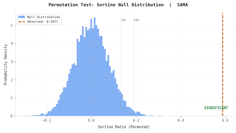
Fig. 1: An illustrative permutation null distribution histogram for a strong strategy variant. The blue null distribution is centered near zero, while the observed Sortino Ratio marker sits far out in the right tail with a green SIGNIFICANT label, indicating a directional edge that chance does not reproduce.

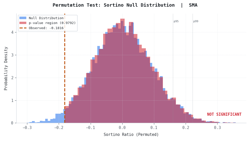
Fig. 2: An illustrative permutation null distribution for a weak strategy variant. The observed Sortino Ratio marker falls inside the body of the null distribution and the chart is labeled NOT SIGNIFICANT, showing that random sign-flipping reproduces this performance level easily.

Section 5: Module B: Bootstrap Confidence Intervals for Key Metrics

The Bootstrap Mechanism

The bootstrap treats the observed trade sample as a proxy for the unknown population of all trades the strategy could have generated. It creates thousands of synthetic samples by drawing trades with replacement from the original sample, so some trades appear twice or more in a given resample and others not at all. Each resample is one plausible alternative realization of the same sample size from the same process. Computing the metric of interest on each resample builds an empirical sampling distribution without any parametric assumptions.

This is meaningful only when trades are treated as exchangeable observations, which holds reasonably well when trade returns are not strongly serially correlated. For mean-reverting systems or strategies with strong momentum in their equity curve, a block bootstrap that preserves local temporal structure is more appropriate than the simple i.i.d. bootstrap implemented here.

Bias-Corrected and Accelerated Intervals

The percentile interval, taking the 2.5th and 97.5th percentiles of the bootstrap distribution, is the simplest approach but can be biased when the sampling distribution of the estimator is skewed. The bias-corrected and accelerated (BCa) interval adjusts for both bias and skewness using a bias-correction term derived from the resample distribution and an acceleration term derived from a jackknife. The implementation reports both the percentile and BCa intervals, defaulting to BCa for the primary result.

Implementation: bootstrap_ci()

def bootstrap_ci(df           : pd.DataFrame,
                 profit_col   : str   = "Trade_Profit_USD",
                 metrics      : list  = None,
                 n_bootstrap  : int   = 10_000,
                 confidence   : float = 0.95,
                 random_seed  : int   = 42) -> pd.DataFrame:
    if metrics is None:
        metrics = ["sortino", "mean_profit", "win_rate",
                   "max_drawdown", "profit_factor"]
    rng     = np.random.default_rng(random_seed)
    profits = df[profit_col].dropna().values.astype(float)
    n       = len(profits)
    if n < 10:
        raise ValueError(f"Bootstrap needs >= 10 trades. Found: {n}.")
    alpha_tail = (1.0 - confidence) / 2.0

    def compute_metric(p: np.ndarray, name: str) -> float:
        if name == "sortino":
            return compute_sortino(p)
        elif name == "mean_profit":
            return float(p.mean())
        elif name == "win_rate":
            return float(np.mean(p > 0) * 100.0)
        elif name == "max_drawdown":
            eq = equity_curve_from_trades(p)
            return max_drawdown_pct_from_equity(eq)
        elif name == "profit_factor":
            gp = p[p > 0].sum()
            gl = abs(p[p < 0].sum())
            return float(gp / gl) if gl > 0 else np.inf
        return 0.0

    rows = []
    for metric in metrics:
        observed  = compute_metric(profits, metric)
        boot_vals = np.array([
            compute_metric(rng.choice(profits, size=n, replace=True), metric)
            for _ in range(n_bootstrap)
        ])
        ci_lo_pct = float(np.percentile(boot_vals, alpha_tail * 100))
        ci_hi_pct = float(np.percentile(boot_vals, (1 - alpha_tail) * 100))

        prop      = np.clip(np.mean(boot_vals < observed), 1e-6, 1 - 1e-6)
        z0        = scipy_stats.norm.ppf(prop)
        jack_vals = np.array([compute_metric(np.delete(profits, j), metric)
                              for j in range(n)])
        jm        = jack_vals.mean()
        num       = np.sum((jm - jack_vals) ** 3)
        den       = 6.0 * (np.sum((jm - jack_vals) ** 2) ** 1.5)
        accel     = num / den if den != 0 else 0.0

        def bca_q(za):
            z_adj = z0 + (z0 + za) / (1 - accel * (z0 + za))
            return float(np.percentile(boot_vals,
                                       scipy_stats.norm.cdf(z_adj) * 100))

        rows.append({
            "Metric"       : metric,
            "Observed"     : round(observed, 4),
            "CI_Lower_Pct" : round(ci_lo_pct, 4),
            "CI_Upper_Pct" : round(ci_hi_pct, 4),
            "CI_Lower_BCa" : round(bca_q(scipy_stats.norm.ppf(alpha_tail)), 4),
            "CI_Upper_BCa" : round(bca_q(scipy_stats.norm.ppf(1-alpha_tail)), 4),
            "Std_Error"    : round(float(boot_vals.std()), 4),
        })
    return pd.DataFrame(rows)

Visualization: CI Comparison Across Indicators

The comparison chart plots the BCa interval for one metric across every indicator variant as a horizontal error-bar chart, sorted by the observed value. A vertical reference line at zero makes it immediately visible which variants retain a positive lower bound. The width of each bar is the visual signature of estimate uncertainty.

def plot_bootstrap_ci_comparison(ci_results_map : dict,
                                 metric         : str  = "sortino",
                                 save_path      : str  = None):
    rows = []
    for indicator, ci_df in ci_results_map.items():
        mask = ci_df["Metric"] == metric
        if not mask.any():
            continue
        row = ci_df.loc[mask].iloc[0]
        rows.append({"Indicator" : indicator, "Observed" : row["Observed"],
                     "Lower" : row["CI_Lower_BCa"], "Upper" : row["CI_Upper_BCa"],
                     "Error_Lo" : row["Observed"] - row["CI_Lower_BCa"],
                     "Error_Hi" : row["CI_Upper_BCa"] - row["Observed"]})
    if not rows:
        return
    plot_df    = pd.DataFrame(rows).sort_values("Observed", ascending=True)
    indicators = plot_df["Indicator"].values
    observed   = plot_df["Observed"].values
    err_lo     = plot_df["Error_Lo"].values
    err_hi     = plot_df["Error_Hi"].values
    palette    = sns.color_palette("deep", len(indicators))
    y_pos      = np.arange(len(indicators))

    fig, ax = plt.subplots(
        figsize=(FIG_WIDTH_IN, max(3.4, len(indicators) * 0.7 + 1.6))
    )
    fig.suptitle(
        f"Bootstrap BCa Confidence Intervals  |  "
        f"{metric.replace('_',' ').title()} by Indicator",
        fontsize=11, fontweight="bold", color=COL_TITLE
    )
    for i, (ind, obs, elo, ehi, color) in enumerate(
        zip(indicators, observed, err_lo, err_hi, palette)
    ):
        ax.errorbar(obs, i, xerr=[[elo], [ehi]],
                    fmt="o", color=color, markersize=7,
                    linewidth=1.8, capsize=5, capthick=1.5,
                    ecolor=color, alpha=0.95)
        ax.text(obs + max(err_hi) * 0.04, i,
                f"{obs:.4f}", va="center", ha="left",
                fontsize=7, color=COL_TEXT)
    ax.axvline(0, color=COL_REF, linewidth=0.9, linestyle=":")
    ax.set_yticks(y_pos)
    ax.set_yticklabels(indicators, fontsize=8)
    ax.set_xlabel(f"{metric.replace('_',' ').title()} (BCa 95% CI)",
                  fontsize=9, labelpad=7)
    ax.grid(axis="x", alpha=0.4)
    ax.spines[["top", "right"]].set_visible(False)
    ax.set_title(
        "Error bars show BCa-corrected 95% bootstrap confidence intervals",
        fontsize=7.5, color=COL_MUTED, style="italic", pad=6
    )
    plt.tight_layout()
    if save_path:
        plt.savefig(save_path, dpi=FIG_DPI, facecolor="#ffffff")
    plt.close(fig)

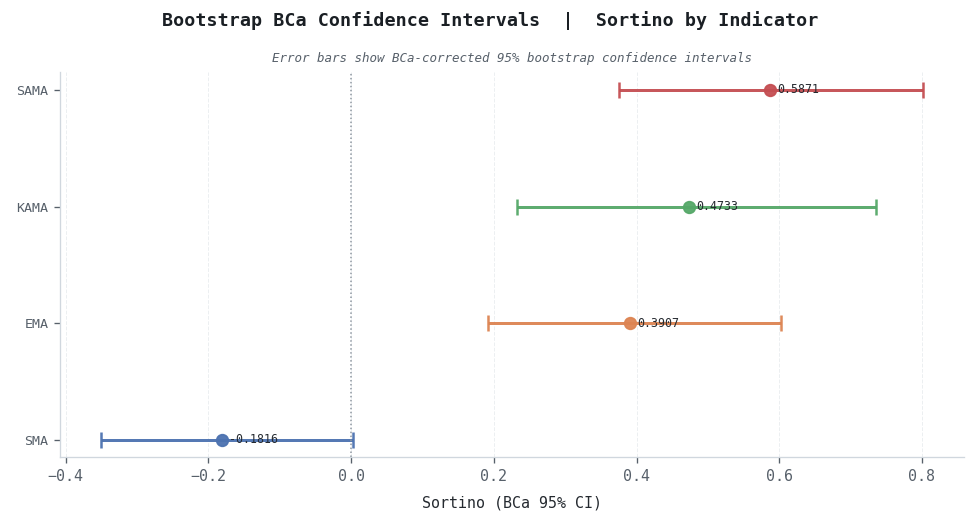
Fig. 3: An illustrative horizontal error-bar chart comparing BCa Sortino Ratio confidence intervals across four indicator variants. The weakest variant's interval crosses the zero reference line while the strongest variants sit entirely to the right of zero.

Section 6: Module C: Monte Carlo Trade-Sequence Shuffling

Why Sequence Matters

Two strategies can have identical sets of trade outcomes, the same wins, the same losses, the same gross P&L, but radically different equity curves and maximum drawdowns depending entirely on the order the trades occurred. A strategy that produced its losing trades early and its winning trades late shows a very different drawdown profile than one with the same trades in reverse order.

The Strategy Tester produces one observed sequence, fixed by the market's actual chronological evolution. Monte Carlo shuffling asks: across all possible orderings of these same trades, where does the observed sequence sit? If the observed drawdown ranks at the 5th percentile of the shuffled distribution, meaning 95% of orderings produce a worse drawdown, then the favorable risk profile is partly attributable to lucky sequencing rather than to the trades themselves. If the observed drawdown sits near the median, the observed sequence is representative.

The Shuffling Mechanism and Equity Reconstruction

Each simulation draws the observed Trade_Profit_USD values in a random order, reconstructs the equity curve as a cumulative sum from a standardized initial equity (default 10,000 USD), and records the maximum drawdown in both absolute and percentage terms. The initial equity is held constant so that results are directly comparable across instruments and lot sizes.

def equity_curve_from_trades(profits        : np.ndarray,
                             initial_equity : float = 10_000.0) -> np.ndarray:
    return initial_equity + np.concatenate([[0.0], np.cumsum(profits)])


def max_drawdown_from_equity(equity: np.ndarray) -> float:
    running_max = np.maximum.accumulate(equity)
    return float((running_max - equity).max())


def max_drawdown_pct_from_equity(equity: np.ndarray) -> float:
    running_max = np.maximum.accumulate(equity)
    dd_pct      = np.where(running_max > 0,
                           (running_max - equity) / running_max * 100.0,
                           0.0)
    return float(dd_pct.max())

The Drawdown Distribution and Percentile Markers

For each shuffle, the percentage drawdown is recorded, and the collection forms the Monte Carlo drawdown distribution. Three markers summarize it. P5 is the drawdown only 5% of orderings would beat; if the observed drawdown is near or below P5, the sequence is exceptionally favorable. P50 is the representative drawdown under a typical ordering. P95 is the stress-test boundary, the drawdown 95% of orderings would not exceed, answering "what should I plan for under adverse sequencing?"

Implementation: monte_carlo_equity_simulation()

def monte_carlo_equity_simulation(
        df              : pd.DataFrame,
        profit_col      : str   = "Trade_Profit_USD",
        n_simulations   : int   = 10_000,
        initial_equity  : float = 10_000.0,
        random_seed     : int   = 42) -> dict:
    rng     = np.random.default_rng(random_seed)
    profits = df[profit_col].dropna().values.astype(float)
    n       = len(profits)
    if n < 5:
        raise ValueError(f"Monte Carlo needs >= 5 trades. Found: {n}.")

    obs_eq      = equity_curve_from_trades(profits, initial_equity)
    obs_dd_usd  = max_drawdown_from_equity(obs_eq)
    obs_dd_pct  = max_drawdown_pct_from_equity(obs_eq)

    store_fan   = n_simulations <= 5_000
    equity_fan  = np.empty((n_simulations, n + 1)) if store_fan else None
    sim_dd_usd  = np.empty(n_simulations)
    sim_dd_pct  = np.empty(n_simulations)

    for i in range(n_simulations):
        sh              = rng.permutation(profits)
        eq              = equity_curve_from_trades(sh, initial_equity)
        sim_dd_usd[i]   = max_drawdown_from_equity(eq)
        sim_dd_pct[i]   = max_drawdown_pct_from_equity(eq)
        if store_fan:
            equity_fan[i] = eq

    pct_levels = [5, 25, 50, 75, 95]
    return {
        "observed_max_dd_usd"   : obs_dd_usd,
        "observed_max_dd_pct"   : obs_dd_pct,
        "simulated_dd_usd"      : sim_dd_usd,
        "simulated_dd_pct"      : sim_dd_pct,
        "observed_equity_curve" : obs_eq,
        "simulated_equity_fan"  : equity_fan,
        "percentiles_usd"       : {p: float(np.percentile(sim_dd_usd, p))
                                   for p in pct_levels},
        "percentiles_pct"       : {p: float(np.percentile(sim_dd_pct, p))
                                   for p in pct_levels},
        "observed_dd_pct_rank"  : float(np.mean(sim_dd_pct <= obs_dd_pct) * 100),
        "n_trades"              : n,
        "n_simulations"         : n_simulations,
        "initial_equity"        : initial_equity,
    }

The equity fan is stored only for 5,000 simulations or fewer. Otherwise, the n_simulations × (n_trades + 1) array can consume excessive memory. The drawdown distribution itself is always computed regardless of the fan.

Visualization: Simulated Equity Fan and Drawdown Envelope

The Monte Carlo chart has two panels. The left panel shows the equity fan: percentile bands across all shuffled curves with the observed path overlaid in orange. The right panel shows the drawdown distribution as a kernel density estimate with percentile markers and the observed drawdown overlaid. The Monte Carlo drawdown histogram also uses an adaptive bin count for safety on low-variance distributions.

def plot_monte_carlo_results(mc_result : dict,
                             indicator : str  = "",
                             save_path : str  = None):
    obs_equity = mc_result["observed_equity_curve"]
    equity_fan = mc_result["simulated_equity_fan"]
    sim_dd_pct = mc_result["simulated_dd_pct"]
    obs_dd_pct = mc_result["observed_max_dd_pct"]
    pct_pct    = mc_result["percentiles_pct"]
    obs_rank   = mc_result["observed_dd_pct_rank"]
    n_trades   = mc_result["n_trades"]
    title_tag  = f"  |  {indicator}" if indicator else ""

    fig, (ax1, ax2) = plt.subplots(1, 2, figsize=(FIG_WIDTH_IN, 4.8))
    fig.suptitle(f"Monte Carlo Trade-Sequence Analysis{title_tag}",
                 fontsize=11, fontweight="bold", color=COL_TITLE)

    x = np.arange(n_trades + 1)
    if equity_fan is not None:
        p5  = np.percentile(equity_fan, 5,  axis=0)
        p25 = np.percentile(equity_fan, 25, axis=0)
        p75 = np.percentile(equity_fan, 75, axis=0)
        p95 = np.percentile(equity_fan, 95, axis=0)
        p50 = np.percentile(equity_fan, 50, axis=0)
        ax1.fill_between(x, p5,  p95,  color=COL_BLUE, alpha=0.12,
                         label="P5-P95 Band")
        ax1.fill_between(x, p25, p75,  color=COL_BLUE, alpha=0.25,
                         label="P25-P75 Band")
        ax1.plot(x, p50, color=COL_BLUE, linewidth=1.2,
                 linestyle="--", alpha=0.80, label="Median Simulated")
    ax1.plot(x, obs_equity, color=COL_ORANGE,
             linewidth=2.0, zorder=5, label="Observed Path")
    ax1.axhline(mc_result["initial_equity"],
                color=COL_REF, linewidth=0.8, linestyle=":")
    ax1.set_xlabel("Trade Number", fontsize=9, labelpad=7)
    ax1.set_ylabel("Equity (USD)", fontsize=9, labelpad=7)
    ax1.set_title("Equity Fan",    fontsize=9, color=COL_MUTED, pad=6)
    ax1.legend(fontsize=7, loc="upper left",
               framealpha=0.85, edgecolor=COL_EDGE)
    ax1.grid(True, alpha=0.4)
    ax1.spines[["top", "right"]].set_visible(False)

    sns.kdeplot(sim_dd_pct, ax=ax2, color=COL_BLUE,
                linewidth=2.0, fill=True, alpha=0.20)
    dd_bins = int(max(10, min(50, len(np.unique(sim_dd_pct)))))
    ax2.hist(sim_dd_pct, bins=dd_bins, density=True,
             color=COL_BLUE, alpha=0.12, edgecolor="none", zorder=0)
    pct_colors = {5:COL_GREEN, 25:COL_AMBER, 50:COL_MUTED,
                  75:COL_AMBER, 95:COL_RED}
    keys_list  = list(pct_pct.keys())
    for pct, val in pct_pct.items():
        ax2.axvline(val, color=pct_colors.get(pct, COL_MUTED),
                    linewidth=0.9, linestyle=":", alpha=0.85)
        ax2.text(val + 0.05,
                 ax2.get_ylim()[1] * (0.88 - 0.12 * keys_list.index(pct)),
                 f"P{pct}:{val:.1f}%",
                 fontsize=6.0, color=pct_colors.get(pct, COL_MUTED),
                 ha="left")
    ax2.axvline(obs_dd_pct, color=COL_ORANGE, linewidth=2.0,
                linestyle="--", label=f"Observed: {obs_dd_pct:.1f}%")
    ax2.set_xlabel("Max Drawdown (%)",     fontsize=9, labelpad=7)
    ax2.set_ylabel("Density",              fontsize=9, labelpad=7)
    ax2.set_title("Drawdown Distribution", fontsize=9, color=COL_MUTED, pad=6)
    ax2.legend(fontsize=7, loc="upper right",
               framealpha=0.85, edgecolor=COL_EDGE)
    rank_color = COL_GREEN if obs_rank <= 30 else (
                 COL_AMBER if obs_rank <= 60 else COL_RED)
    ax2.text(0.97, 0.08,
             f"Observed DD @ P{obs_rank:.0f}\nof simulated distribution",
             transform=ax2.transAxes, fontsize=7.5,
             color=rank_color, ha="right", va="bottom",
             bbox=dict(boxstyle="round,pad=0.3",
                       facecolor="#f6f8fa",
                       edgecolor=COL_EDGE, alpha=0.95))
    ax2.grid(True, alpha=0.4)
    ax2.spines[["top", "right"]].set_visible(False)
    plt.tight_layout()
    if save_path:
        plt.savefig(save_path, dpi=FIG_DPI, facecolor="#ffffff")
    plt.close(fig)

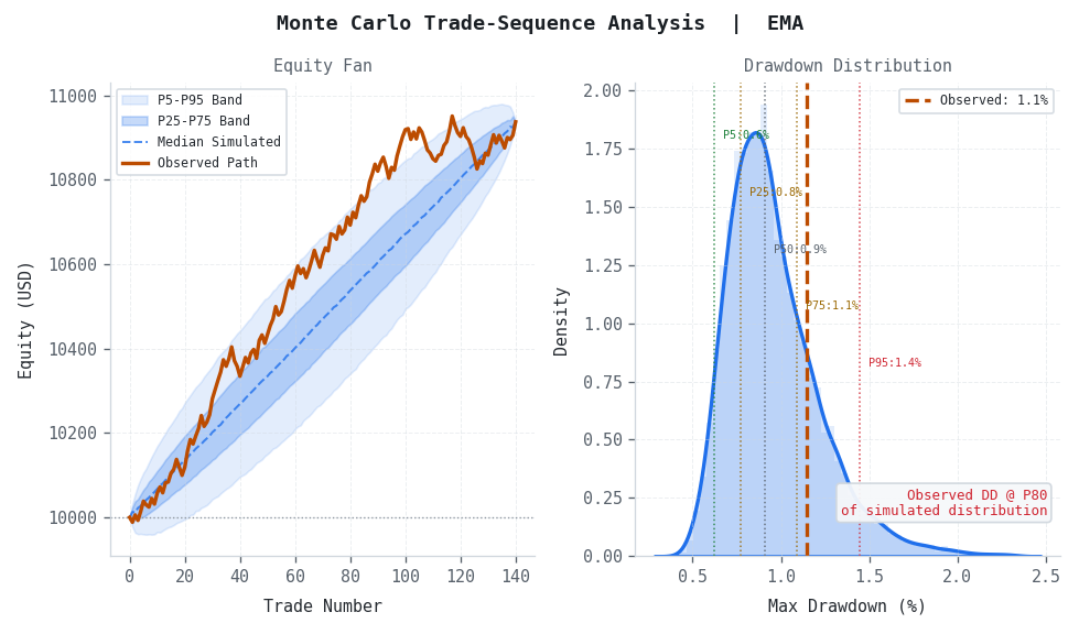
Fig. 4: An illustrative two-panel Monte Carlo chart. The left panel shows the observed equity path in orange tracking through the blue percentile bands of all shuffled orderings. The right panel shows the drawdown distribution with P5, P50, and P95 markers and the observed drawdown annotated with its percentile rank.

Section 7: The Unified Robustness Report

The three modules produce independent outputs. The unified battery runs all three against every indicator variant in the dataset and writes a structured summary to disk. The CSV reader uses a flexible encoding fallback so that ANSI-encoded MetaTrader exports load correctly on Windows, macOS, and Linux, since the ansi codec alias exists only on Windows.

def _read_csv_flexible(path: str) -> pd.DataFrame:
    """
    Reads a CSV produced by the MQL5 exporter. MetaTrader writes ANSI
    encoded files. On Windows the 'ansi' alias resolves natively; on
    other platforms it is not a known codec, so this helper tries a
    sequence of encodings and returns the first that succeeds.
    """
    for enc in ("cp1252", "utf-8", "latin-1"):
        try:
            return pd.read_csv(path, encoding=enc)
        except (UnicodeDecodeError, LookupError):
            continue
    return pd.read_csv(path, encoding="latin-1")


def run_robustness_battery(
        trade_csv_path  : str,
        output_dir      : str   = "robustness_outputs",
        n_permutations  : int   = 10_000,
        n_bootstrap     : int   = 10_000,
        n_monte_carlo   : int   = 5_000,
        alpha           : float = 0.05,
        random_seed     : int   = 42) -> pd.DataFrame:

    os.makedirs(output_dir, exist_ok=True)
    if not os.path.isfile(trade_csv_path):
        raise FileNotFoundError(f"Trade CSV not found: {trade_csv_path}")
    df = _read_csv_flexible(trade_csv_path)
    if "Trade_Profit_USD" not in df.columns:
        raise ValueError("Column 'Trade_Profit_USD' not found.")

    indicators     = (df["Indicator_Name"].unique()
                      if "Indicator_Name" in df.columns
                      else ["All_Trades"])
    summary_rows   = []
    ci_results_map = {}

    for indicator in indicators:
        print(f"\n[Robustness] Testing: {indicator}")
        subset = (df[df["Indicator_Name"] == indicator].copy()
                  if "Indicator_Name" in df.columns else df.copy())
        if len(subset) < 10:
            print(f"  [Skip] Insufficient trades ({len(subset)}).")
            continue

        perm_result = permutation_test(
            subset, n_permutations=n_permutations,
            alpha=alpha, random_seed=random_seed)
        plot_permutation_null(
            perm_result, indicator=indicator,
            save_path=os.path.join(output_dir,
                                   f"Permutation_Null_{indicator}.png"))

        ci_df = bootstrap_ci(
            subset, n_bootstrap=n_bootstrap, random_seed=random_seed)
        ci_results_map[indicator] = ci_df
        ci_df.to_csv(os.path.join(output_dir,
                                  f"Bootstrap_CI_{indicator}.csv"),
                     index=False)

        mc_result = monte_carlo_equity_simulation(
            subset, n_simulations=n_monte_carlo, random_seed=random_seed)
        plot_monte_carlo_results(
            mc_result, indicator=indicator,
            save_path=os.path.join(output_dir,
                                   f"MonteCarlo_{indicator}.png"))

        sortino_ci = (ci_df[ci_df["Metric"] == "sortino"].iloc[0]
                      if not ci_df[ci_df["Metric"] == "sortino"].empty
                      else None)
        summary_rows.append({
            "Indicator"             : indicator,
            "N_Trades"              : perm_result["n_trades"],
            "Observed_Sortino"      : perm_result["observed_sortino"],
            "Permutation_P_Value"   : perm_result["p_value"],
            "Permutation_Sig"       : perm_result["significant"],
            "Bootstrap_Sortino_Lo"  : (sortino_ci["CI_Lower_BCa"]
                                       if sortino_ci is not None else None),
            "Bootstrap_Sortino_Hi"  : (sortino_ci["CI_Upper_BCa"]
                                       if sortino_ci is not None else None),
            "MC_Obs_DD_Pct"         : mc_result["observed_max_dd_pct"],
            "MC_DD_P50"             : mc_result["percentiles_pct"][50],
            "MC_DD_P95"             : mc_result["percentiles_pct"][95],
            "MC_Obs_DD_Rank"        : mc_result["observed_dd_pct_rank"],
        })
        print(f"  {perm_result['interpretation']}")

    if len(ci_results_map) > 1:
        plot_bootstrap_ci_comparison(
            ci_results_map, metric="sortino",
            save_path=os.path.join(output_dir,
                                   "Bootstrap_CI_Comparison_Sortino.png"))

    summary_df = pd.DataFrame(summary_rows)
    summary_df.to_csv(os.path.join(output_dir, "Robustness_Summary.csv"),
                      index=False)
    return summary_df

Section 8: Testing the Pipeline Without a Live Export

A reader who has not yet produced a MetaTrader export can still run the full battery using a synthetic data generator, generate_sample_trades.py. It writes a CSV in the exact schema the battery consumes, populated with four indicator profiles of deliberately different quality: a weak near-random variant, a modest genuine edge, a strong but volatile edge, and a strong consistent edge. This lets the battery be exercised end to end and, more importantly, lets you confirm that the tests actually distinguish a real edge from noise, rather than merely run without errors.

The recommended testing sequence is three commands:

pip install numpy pandas scipy matplotlib seaborn
python generate_sample_trades.py     # writes exports/trade_level_results.csv
python robustness_testing.py         # reads that file, writes robustness_outputs/

On the synthetic data, the weak variant correctly reads as not significant with a Sortino Ratio confidence interval that crosses zero, while the three genuine-edge variants register as highly significant with positive lower bounds. Confirming this expected pattern is the verification that the battery is behaving correctly before it is pointed at real strategy data. To switch to real data, replace the synthetic CSV with the file produced by the demo EA from Section 4 and rerun the battery unchanged.

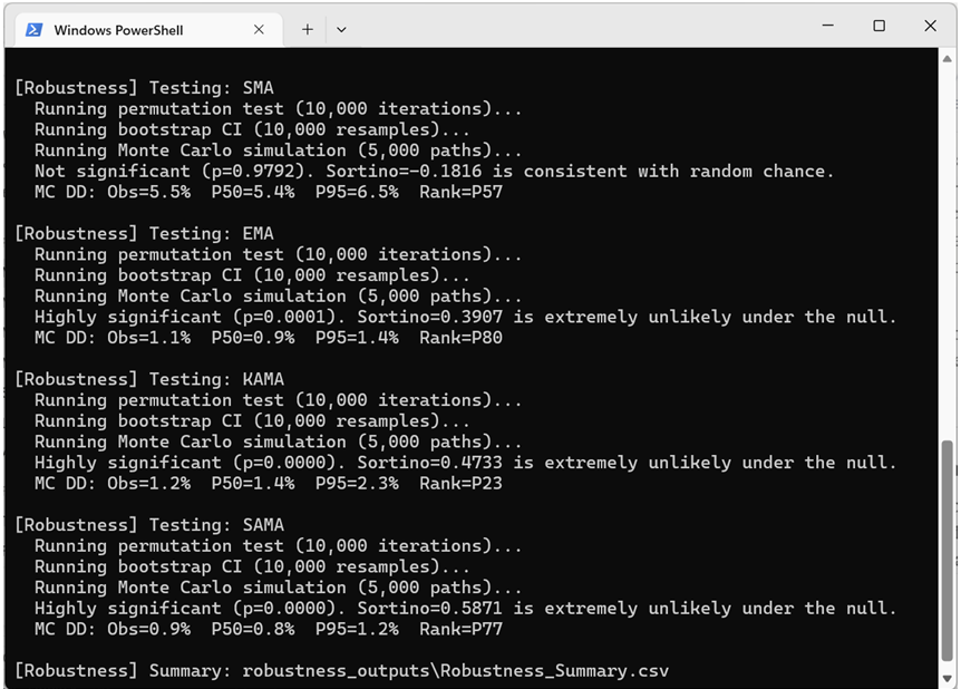
Fig. 5: Windows PowerShell output from a full battery run on the synthetic dataset, showing the per-indicator interpretation lines: the weak variant labeled not significant and the three edge variants labeled highly significant.

Section 9: Interpreting Robustness Results: A Decision Framework

The three tests produce five primary outputs per indicator: a permutation p-value, two bootstrap CI bounds on the Sortino Ratio, the observed drawdown percentile rank, and the P95 stress-test drawdown. A strategy passes the robustness battery when all five conditions hold:

1. Permutation p-value below 0.05: The Sortino Ratio is statistically distinguishable from a no-edge null.
2. Bootstrap Sortino Ratio CI lower bound positive: Even at the pessimistic end of the interval, the strategy retains a positive risk-adjusted return.
3. Bootstrap Sortino Ratio CI narrow relative to the observed value: A CI spanning 0.8 to 2.4 against an observed 1.6 signals high sampling uncertainty; a CI spanning 1.3 to 1.9 signals stability.
4. Observed drawdown ranks at or below the 40th percentile of the Monte Carlo distribution: The observed sequence is not anomalously favorable relative to typical orderings.
5. P95 stress-test drawdown within the strategy's risk tolerance: If the maximum acceptable drawdown is 20% and the P95 Monte Carlo drawdown is 35%, the strategy will breach tolerance under roughly 5% of plausible orderings.

A strategy that fails any one condition warrants investigation rather than immediate rejection. A marginal permutation result on a short trade history may reflect insufficient statistical power rather than absence of edge. A wide bootstrap CI on a volatile strategy may narrow substantially with more data. A high observed drawdown rank may reflect that the test period happened to include an unusually adverse drawdown sequence. The tests surface these conditions for investigation; they do not replace the practitioner's domain judgment.

When the battery has been run for several variants on the same instrument and timeframe, Robustness_Summary.csv provides a structured comparison across all five dimensions at once. A developer can rank by Permutation_P_Value, filter to only those with Permutation_Sig == True, and within that filtered set rank by MC_Obs_DD_Rank to find which variant's observed drawdown is most representative of its trade distribution rather than the product of favorable sequencing.

Conclusion

This article established a validation framework designed to differentiate a genuine structural edge from a statistically random backtest. The underlying architecture enforces a five-condition survival criterion across three modules: a sign-randomization permutation test to evaluate if an observed Sortino Ratio could occur without a directional edge, a bootstrapping component that replaces single point estimates with stability confidence intervals, and a Monte Carlo simulation to isolate sequence dependency from actual drawdown characteristics. To make this rigor reproducible, an automated pipeline ingests an EA-generated trade-level CSV file via a minor code integration, executing the full analytical battery to produce standardized 980-pixel charts and a consolidated summary table.

The framework quantifies validity for the tested period. It cannot guarantee future profitability, anticipate regime shifts, or account for execution friction and overfitting. Its primary utility lies in mitigating the risk of deploying a strategy optimized purely by chance, identifying statistical failures cheaply before live capital is committed. Passing this evaluation battery establishes historical performance integrity, verifying that the strategy has earned the right to subsequent out-of-sample testing.

Programs used in the article

#	Name	Type	Description
1	TradeLevelExport.mqh	Include File	Connects a live EA to the Python analytics. Iterates the deal history, matches each exit deal to its entry by position ID, and writes one row per closed trade in the schema the battery expects. Uses the spin-lock open pattern from Part 1.
2	RobustnessDemoEA.mq5	Demo EA	A minimal EMA-crossover EA showing how to connect the export include. Tags orders with a magic number in OnInit() and calls ExportTradeLevelCSV() from OnDeinit() inside the tester, illustrating the three integration touch points.
3	robustness_testing.py	Python Script	The core analytics module. Runs three robustness tests per indicator variant: a sign-randomization permutation test on the Sortino Ratio, BCa bootstrap confidence intervals, and Monte Carlo trade-sequence shuffling. Writes charts, CI tables, and a summary CSV. Charts render on white at 980px, with cross-platform CSV encoding support.
4	generate_sample_trades.py	Python Script	A synthetic data generator for testing the battery without a live export. Writes a CSV in the export schema with four indicator profiles of differing quality, so each module produces a verifiable result.
5	CSV_Data_Analysis_Part_7.zip	Zip Archive	Zip archive containing all the attached files and their paths relative to the terminal's root folder.