Coyote Optimization Algorithm (COA)
 82
 0

Contents
Introduction
Anyone who has ever run a trading system optimization knows that feeling. The parameter space is vast: indicator periods, stop-loss and take-profit levels, time and volatility filters — even a simple Expert Advisor can easily have a dozen dimensions. An exhaustive search is physically impossible. Premature convergence is the main enemy of anyone seeking stable parameters in a multimodal landscape, and the profit landscape of a trading system is precisely that: rugged, noisy, and full of narrow peaks and broad, gentle plateaus — which are actually what interest us most.
We have an optimization problem, and we know that relying on a single swarm converging to a single point is a gamble. This raises the question: Are there algorithms that can explore multiple regions of space in parallel without sacrificing convergence speed? In our series of articles on population-based optimization algorithms, we have already examined dozens of metaheuristics — from classic swarm-based algorithms to the most exotic ones — and run each through the same test bench: the Hilly, Forest, and Megacity functions, three problem dimensionalities, a fixed budget of 10,000 calls to the objective function, and ten repetitions. This standardized protocol lets us compare all the algorithms under equal conditions rather than taking their developers at their word. The series' ranking table has shown time and again that a catchy name and an appealing metaphor from nature are no guarantee of success.
Today's guest in the series is the Coyote Optimization Algorithm (COA), proposed by Juliano Pierezan and Leandro dos Santos Coelho in 2018. At first glance, it is just another animal in the sprawling zoo of metaheuristics. But COA has a distinctive structural feature: its population is divided from the outset into isolated packs, each of which leads its own social life, evolves around its own leader, and only occasionally exchanges individuals with its neighbors. It is not a swarm that breathes as a single entity — it is an archipelago of small populations that naturally preserves diversity. There are also two mechanisms absent from a typical swarm: the pack's collective culture, expressed through the median (rather than the mean — and this matters), and the birth of pups — genetic crossover built directly into the swarm-based scheme.
By the end of this article, the reader will have an understanding of the social mechanics of COA, a ready-to-use class implementation within the standard C_AO architecture with an explanation of all adaptations of the original authors’ sequential scheme to our test bench, honest results across the full set of functions, and the algorithm’s position in the series’ ranking table. Along the way, the reader will also get an answer to a practical question: does the pack structure offer a real advantage in maintaining diversity, or is it merely an attractive wrapper around an ordinary swarm? First, we will break down the concept and the math behind the algorithm using real-life examples, then implement it in MQL5, discuss the pitfalls of porting it, and test the result on the test bench.
Implementation of the Algorithm
Metaphor: not a swarm, but a society
Most swarm algorithms simulate a crowd: all agents see the global leader and move toward it. COA models something more complex — a society with a social structure.
In the wild, coyotes live in packs of several individuals. Every pack has an alpha — the fittest individual. The pack also has collective experience — its culture: a set of behaviors that belongs to no single individual but is shared by all. Coyotes learn from one another; pups are born in packs and inherit their parents’ traits; and sometimes an individual leaves one pack to join another, bringing its accumulated experience with it.
To put this in a trader's terms, imagine not just one team of trading system developers, but several independent teams. Each team has its own leader with the best current performance and its own school of thought — a trading style typical of that team. There is a constant exchange of ideas within the team; from time to time, hybrid strategies emerge — pieced together from parts of two other strategies — and occasionally a trader moves from one team to another, bringing a fresh perspective with them. Several teams will almost certainly explore different trading ideas; one large team will almost certainly settle on just one. Now, let's talk about the mechanisms.
Coyote = solution, pack = subpopulation. Each coyote is a vector of problem parameters — that is, a candidate solution: in our terminology, a specific set of trading system parameters. A coyote's social state is its position in the search space; its fitness is the value of the objective function.
A population of popSize coyotes is divided into nPacks packs, each containing nCoy individuals (the authors use 20 packs of 5 coyotes each). The grouping is random and — crucially — remains almost unchanged: the packs are not re-sorted by fitness at every iteration, as in some algorithms with castes. The composition of the pack changes only on rare occasions when an exchange takes place, as discussed below. It is precisely this stable isolation that allows packs to disperse across different areas of the landscape.
Alpha and pack culture. At each iteration, two reference points are determined for each pack. The first is the alpha: the best coyote in the pack in terms of fitness. This is the equivalent of a local leader — not a global one! Each pack looks up to its own champion, not the world champion. If one pack finds a high peak, the others do not abandon their areas and continue digging where they are. The second is the pack's social tendency: the coordinate-wise median of the positions of all its coyotes. This is the formalization of culture — a generalized portrait of the pack that does not correspond to any single individual.
Why the median rather than the mean — that is a detail worth considering. Imagine a team of five traders, four of whom trade using a moving average with a period of about 20, while the fifth — an experimenter — uses a period of 200. The arithmetic mean comes out to 56 — a value that no one uses in trading and that reflects neither the consensus nor the experiment. The median gives 20 — an honest reflection of “how things are done on this team.” The median is resistant to outliers: a single coyote that has strayed to the edge of the space does not drag the entire pack’s culture along with it. In an algorithm where outliers are a normal result of exploration, this is a deliberate engineering decision.
Social move: learning from the leader and the environment. Primary movement operator. Every coyote in the pack (except for one — its place will be taken by a pup, as explained below) builds a new social state according to the following formula:
new = x + r1 * (alpha - x_rc1) + r2 * (tend - x_rc2)
where:
- x — the coyote's current position,
- alpha — the alpha's position,
- tend — the pack's cultural tendency,
- x_rc1 and x_rc2 are two randomly selected pack members from the same pack (distinct from each other and from the coyote itself),
- r1, r2 are random numbers from [0, 1].
Let's break down what is actually happening here. The coyote takes two steps at once. The first is what I learn from the leader: the vector (alpha - x_rc1) shows how far and in which direction the alpha differs from a randomly selected ordinary pack member. Second — what my environment teaches me: the vector (tend - x_rc2) shows how much a random pack member deviates from the cultural norm and pulls toward that norm.
A real-life example: You are a trader on a team. You look at the leader and a randomly selected colleague and think, “The leader's stop-loss is half as wide as Petya's — I will try tightening mine, too.” Then you look at the team's usual practice and another colleague: “On our team, we apply a filter to Asian-session trading, but Vasya does not — I suppose I am closer to the team's practice.” Importantly, in both cases the reference point is not the learner itself, but randomly selected pack members. This introduces a stochastic component into the step that depends on the current spread of the pack — as long as the pack is spread out, the steps are large; when the pack contracts around a peak, the steps automatically become smaller. A simple, built-in mechanism for transitioning from exploration to refinement, without any coefficients that decay with the iteration number.
Acceptance of a new state is greedy and strict: a coyote moves to a new point only if it is better than the previous one. No accepting worse solutions for the sake of diversity — other mechanisms handle diversity in COA.
Birth of a Pup: Genetics Within the Swarm
The most unusual part of the algorithm. Once per iteration, a pup is born in each pack — a new solution assembled from the genes of two randomly selected parents who are pack members, plus fresh random material.
Here's how it works. Two different parents are selected at random. Next, each coordinate's fate is decided: it is inherited from the first parent, inherited from the second, or generated randomly anew (mutation). The algorithm ensures that at least one coordinate is taken from the first parent and at least one from the second: the pup cannot be a pure clone or an entirely random solution. The mutation probability for each coordinate is Ps = 1/D, where D is the dimensionality of the problem, so on average one coordinate mutates per pup, regardless of dimensionality; otherwise, the coordinate is inherited from either parent with equal probability, (1 - Ps)/2 for each.
In trading system terms: let’s take Masha’s system and Igor’s system. For the new system, the channel period comes from Masha, the take-profit coefficient comes from Igor, the volatility filter comes from Masha, and we randomly select the trading session time. The result is a hybrid that no one had before — and sometimes such a hybrid really takes off where both parents were mediocre, because a successful combination of parameters does not necessarily lie on the line segment between two successful solutions. The social move is a continuous operator: it can move along directions; crossover is a combinatorial operator: it can jump to corners of the space that smooth motion cannot reach. In COA, they work together — a combination rarely found in swarm algorithms.
A pup's fate is determined by natural selection: it takes the place of the worst-performing coyote in the pack — if it proves to be better than that coyote. This is where age comes into play: all else being equal, the oldest of the worst-performing coyotes is replaced. The age of all coyotes increases by one each iteration; a newborn pup starts at zero. The pack slowly but continuously rejuvenates, and veterans whose progress has stalled cannot keep their places forever just because of their seniority.
Inter-pack exchange: rare, but important. If the packs were completely isolated, the algorithm would degenerate into a set of independent small optimizations — each with its own budget and its own dead ends. The authors introduce a limited communication channel: with a probability of p_leave = 0.005 * nCoy² per iteration, two randomly selected coyotes from two randomly selected packs swap places.
With a standard pack size of 5 coyotes, this works out to 0.125 — the exchange occurs approximately once every eight iterations. Rarely enough for the packs to retain their individual identities, and often enough for a discovery made by one pack to eventually migrate to its neighbors. This is the very same archipelago model from the theory of island genetic algorithms: isolation preserves diversity, while migration spreads success. Note the quadratic dependence on pack size — the authors calibrated the exchange rate so that large packs, which have more than enough internal diversity, would exchange members more frequently and avoid stagnation.
Putting the Whole Picture Together
A "year" in the life of a population looks like this. Within each pack: the alpha was identified, the cultural median was calculated, each coyote made a social move with greedy acceptance, and a pup was born and competed for a place in the pack. Between packs: a pair of individuals may have been exchanged. Everyone is a year older. The best solution across all packs is the algorithm's current output.
This scheme clearly illustrates the division of labor among the mechanisms: the social move handles local refinement and convergence, pup crossover enables combinatorial leaps and major discoveries, the pack structure maintains multiple search regions in parallel, exchange spreads success, and age drives membership turnover. None of the operators duplicates another — a welcome rarity for an algorithm devised in 2018, at a time when new metaheuristics were churned out simply by renaming old ones.
The test bench will show just how well this design works in practice. In the meantime, let's move on to the implementation in MQL5 and look at the areas where we had to carefully adapt the original sequential scheme to our C_AO architecture.
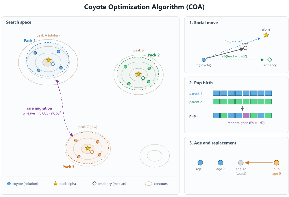
Figure 1. The Coyote Optimization Algorithm: The Social Structure of Search
In the illustration, the population is divided into isolated packs, each of which occupies its own region of the multimodal landscape. Each pack follows its own alpha (the pack’s best coyote) rather than a single global leader, which naturally preserves diversity. A pack’s social tendency is the coordinate-wise median of its members; unlike the mean, it is resistant to outliers. Rare migration (probability p_leave = 0.005·nCoy² per iteration, approximately once every 8 iterations when nCoy = 5) swaps two coyotes between two random packs, spreading successful traits throughout the archipelago.
-
Social movement: Each coyote simultaneously takes a step toward the alpha and toward the pack culture, using two random pack members (rc1 and rc2) as reference points; a new position is adopted only if it strictly improves the solution.
-
Pup birth: Once per iteration, each pack produces a pup through binary crossover between two randomly selected parents — at least one gene is guaranteed to be inherited from each parent, and each gene mutates to a new random value with probability Ps = 1/D.
-
Age and replacement: Each coyote ages by one unit per iteration; a pup replaces the worst coyote in the pack (the oldest in the event of a fitness tie) only if the pup is better, so the pack is continually rejuvenated without losing quality.
Pseudocode for the COA algorithm:
popSize, nCoy, nPacks = popSize/nCoy, coords    — sizes
pLeave  = 0.005 * nCoy^2                        — pack exchange probability (Eq. 4)
Ps      = 1/coords                              — pup coordinate mutation probability
probPup = (1 - Ps)/2                            — coordinate inheritance probability
x[i], f[i]                                      — coyote coordinates and fitness
snap_c[i], snap_f[i]                            — state at the start of the epoch
age[i], isPup[i]                                — coyote age and pup flag
pack[p]                                         — indices of the nCoy coyotes in pack p
cB, fB                                          — globally best coordinates and fitness

INIT
StandardInit(rangeMin, rangeMax, rangeStep)
pLeave  = 0.005 * nCoy^2;   probPup = (1 - 1/coords)/2
for i, c:  cP[i][c] = random_uniform(rangeMin[c], rangeMax[c])   # initial population
age[*] = 0;  isPup[*] = false
indices = shuffle([0 .. popSize-1])                              # Fisher–Yates
distribute the shuffled indices among[0..nPacks-1], with nCoy indices per pack

MOVING
if first pass:                       # only cP → c, so that the test bench can evaluate FF
    for i, c:  x[i][c] = bring_into_range(cP[i][c])
    return

for i:  snap_c[i] = x[i];  snap_f[i] = f[i]      # 1. epoch starting point

if nPacks > 1 and random() < pLeave:             # 2. rare exchange between packs (Eq. 4)
    exchange pack[p1][c1] <-> pack[p2][c2]  for random p1!=p2, c1, c2

isPup[*] = false

for p = 0 .. nPacks-1:                            # 3. operations inside the pack
    alpha = argmax_{k in pack[p]} snap_f[k]               # pack alpha (Eq. 5)
    for c:  tend[c] = median_{k in pack[p]} snap_c[k][c]  # social tendency = median (Eq. 6)
    pup_slot = worst by snap_f (if equal — older by age)   # pup slot
    isPup[pup_slot] = true

    for each i from pack[p]:
        if i == pup_slot:                         # PUP BIRTH (Eq. 7, Alg. 1)
            select two different parents par1, par2 from the pack
            pdr = shuffle([0 .. coords-1])
            mask[*] = 0;  mask[pdr[0]] = 1;  mask[pdr[1]] = 2    # minimum 1 from each
            for j = 2 .. coords-1:
                r = random()
                if   r < probPup:      mask[pdr[j]] = 1
                elif r > 1 - probPup:  mask[pdr[j]] = 2          # otherwise 0 = mutation
            for c:
                v = (mask[c]==1) ? snap_c[par1][c] :
                    (mask[c]==2) ? snap_c[par2][c] :
                                   random_uniform(rangeMin[c], rangeMax[c])
                x[i][c] = bring_into_range(v)
        else:                                     # SOCIAL MOVE (Eq. 12)
            select rc1, rc2 from the pack (both != i, rc1 != rc2)
            r1 = random();  r2 = random()                       # scalars per agent
            for c:
                v = snap_c[i][c]
                  + r1*(snap_c[alpha][c] - snap_c[rc1][c])      # attraction to the leader
                  + r2*(tend[c]          - snap_c[rc2][c])      # attraction to pack culture
                x[i][c] = bring_into_range(v)

After Moving the test bench evaluates f[i] for all agents — exactly popSize FF calls.

REVISION
for i:                                            # updating the best solutions
    update the personal best if f[i] is higher
    if f[i] > fB:  fB = f[i];  cB = x[i]

if first_pass:  revision = true;  return

for i:                                            # adaptation (Eq. 14): greedy acceptance
    accepted = (f[i] > snap_f[i])
    if not accepted:  x[i] = snap_c[i];  f[i] = snap_f[i]      # rollback to the starting point
    age[i]++
    if isPup[i] and accepted:  age[i] = 0                      # a pup's age is reset to zero

EXTERNAL LOOP (stand)
Init();  Moving();  evaluate f[*];  Revision()
for epoch = 1 .. epochCount:
    Moving();  evaluate f[*];  Revision()
response = cB (fitness fB)
Now for the implementation. The C_AO_COA_Coyote class inherits from the base C_AO class and implements the Coyote Optimization Algorithm within the standard architecture used in this series: all iteration logic is split between two methods — Moving (generating new candidates) and Revision (deciding whether to accept candidates and updating the best solutions) — which the test bench’s outer loop calls in turn at each epoch. The base class is not modified.
The user-configurable parameter 'nCoy' specifies the number of coyotes in a pack and, together with the inherited popSize, determines the auxiliary variable nPacks = popSize / nCoy — the number of packs. The parameters pLeave (the probability of individual exchange between packs, equal to 0.005·nCoy²) and probPup (the probability that a pup will inherit a coordinate, equal to (1−1/coords)/2) are calculated once in 'Init', since they depend only on 'nCoy' and the dimensionality.
The composition of the packs is stored in a flat array 'packs' of length 'nPacks·nCoy': the indices of the coyotes belonging to pack 'p' lie in the slice packs[p·nCoy .. p·nCoy+nCoy−1]. The 'ages' array stores the age of each coyote, and 'isPup' marks the slot occupied by a pup in the current epoch.
A snapshot of the population's state at the beginning of the epoch is stored in snap_c (a flat coordinate buffer, popSize·coords) and snap_f (fitness values, popSize) — all moves in the epoch are calculated relative to this snapshot, and rejected candidates are rolled back to it. The working buffers medBuf (for calculating the pack median), tend (social tendency), pdr (permutation of dimensions when a pup is born), and mask (the source of each coordinate of the pup) are reused and do not retain state between epochs.
The constructor sets the algorithm's identifying information (ao_name, ao_desc, and a link to the article) and default values: popSize = 20, nCoy = 5. It registers two configurable parameters in the params array and immediately calculates nPacks so that the object is consistent even before SetParams is explicitly called.
SetParams reads popSize and nCoy from the params array (where an external script places them before execution) and recalculates nPacks = popSize / nCoy. popSize is intentionally left unadjusted: it is an external parameter that the user is responsible for setting to a multiple of nCoy.
//+------------------------------------------------------------------+
//|                            Class                                 |
//+------------------------------------------------------------------+
class C_AO_COA_Coyote : public C_AO
 {
public:
                    ~C_AO_COA_Coyote() {}
                     C_AO_COA_Coyote()
   {
    ao_name = "COA(Coyote)";
    ao_desc = "Coyote Optimization Algorithm";
    ao_link = "https://www.mql5.com/en/articles/23053";

    popSize = 20;
    nCoy    = 5;

    ArrayResize(params, 2);
    params [0].name = "popSize";
    params [0].val = popSize;
    params [1].name = "nCoy";
    params [1].val = nCoy;

    nPacks = popSize / nCoy;
   }

  void               SetParams()
   {
    popSize = (int)params [0].val;
    nCoy    = (int)params [1].val;

    nPacks = popSize / nCoy;
   }

  bool               Init(const double &rangeMinP  [],
                          const double &rangeMaxP  [],
                          const double &rangeStepP [],
                          const int     epochsP = 0);

  void               Moving();
  void               Revision();

  //--- visible parameters
  int                nCoy;       // coyotes in a pack (original: 5)

private:
  int                nPacks;     // number of packs = popSize / nCoy
  double             pLeave;     // probability of exchange between packs: 0.005*nCoy^2
  double             probPup;    // (1 - Ps)/2, where Ps = 1/coords

  int                packs  [];  // [nPacks * nCoy] — agent indices grouped by pack
  int                ages   [];  // [popSize] — coyote age
  bool               isPup  [];  // [popSize] — pup slot in the current epoch

  //--- snapshot for greedy acceptance
  double             snap_c [];  // [popSize * coords]
  double             snap_f [];  // [popSize]

  //--- working buffers
  double             medBuf [];  // [nCoy]   — for the median
  double             tend   [];  // [coords] — pack's social tendency
  int                pdr    [];  // [coords] — permutation of dimensions (pup)
  int                mask   [];  // [coords] — 0: noise, 1: parent 1, 2: parent 2
 };
Initialization prepares the algorithm for a new run. First, it calls the base class's StandardInit method (which allocates the population a[] and stores the search bounds), then populates the proposal buffer cP[] with random coordinates for the initial population. On the first call to Moving, these coordinates will be transferred to the working coordinates c[]. Here, pLeave and probPup are calculated, all auxiliary buffers are allocated, and all ages and pup flags are reset to zero. The method concludes by randomly dividing the population into packs: the indices 0..popSize−1 are shuffled using the Fisher–Yates algorithm and placed in packs.
//+------------------------------------------------------------------+
//|                              Init                                |
//+------------------------------------------------------------------+
bool C_AO_COA_Coyote::Init(const double &rangeMinP  [],
                    const double &rangeMaxP  [],
                    const double &rangeStepP [],
                    const int     epochsP = 0)
 {
  if(!StandardInit(rangeMinP, rangeMaxP, rangeStepP))
    return false;

//--- initial random population in cP[] (Eq. 2)
  for(int i = 0; i < popSize; i++)
    for(int c = 0; c < coords; c++)
      a [i].cP [c] = u.RNDfromCI(rangeMin [c], rangeMax [c]);

//--- parameters that depend on nCoy and coords
  pLeave  = 0.005 * (double)nCoy * (double)nCoy;          // Eq. 4
  probPup = (coords > 0) ? (1.0 - 1.0 / (double)coords) * 0.5 : 0.0; // (1-Ps)/2

//--- buffers
  ArrayResize(snap_c, popSize * coords);
  ArrayResize(snap_f, popSize);
  ArrayResize(packs,  nPacks * nCoy);
  ArrayResize(ages,   popSize);
  ArrayResize(isPup,  popSize);
  ArrayResize(medBuf, nCoy);
  ArrayResize(tend,   coords);
  ArrayResize(pdr,    coords);
  ArrayResize(mask,   coords);

  ArrayInitialize(ages, 0);
  ArrayInitialize(isPup, false);

//--- random distribution of coyotes among packs (Fisher–Yates)
  for(int i = 0; i < popSize; i++)
    packs [i] = i;
  for(int j = popSize - 1; j > 0; j--)
   {
    int r     = u.RNDminusOne(j + 1);
    int tmp   = packs [j];
    packs [j] = packs [r];
    packs [r] = tmp;
   }

  return true;
 }
Moving generates new candidates for all agents in a single epoch without calling the objective function (which is evaluated by the outer loop after returning from the method). On the first run (revision == false), the method simply transfers the initial population from cP[] to the working coordinates c[], snapping the coordinates to the grid and enforcing the bounds, and then exits — this allows the test bench to evaluate the initial population.
In subsequent epochs, the method proceeds as follows: it takes a snapshot of the current population in snap_c / snap_f; with probability pLeave, it swaps two randomly selected coyotes, one from each of two randomly selected packs (migration, Eq. 4); clears the pup flags. It then determines the alpha for each pack (the coyote with the maximum snapshot fitness, Eq. 5), calculates the social tendency as the coordinate-wise median of the pack members (Eq. 6) and assigns the pup slot to the coyote with the lowest fitness score; in the event of a tie, the oldest one is chosen.
After that, each coyote in the pack is assigned a new candidate. The coyote in the pup slot is reborn (Eq. 7, Alg. 1): two distinct parents are selected, the dimensions are shuffled, and, according to a mask, each coordinate is taken from the first parent, taken from the second parent, or generated at random (mutation with probability 1/coords), with each parent guaranteed to contribute at least one coordinate. The remaining coyotes make a social move (Eq. 12): attraction to the alpha and attraction to the pack's social tendency are added to the snapshot position, scaled by the scalars r1 and r2, respectively, randomly sampled for each agent. All new coordinates are adjusted to satisfy the search bounds and align with the search grid.
//+--------------------------------------------------------------------+
//|                            Moving                                  |
//|                                                                    |
//|  Epoch structure:                                                  |
//|    1. Population snapshot;                                         |
//|    2. Infrequent exchange of coyotes between packs (Eq. 4);        |
//|    3. For each pack: alpha, social tendency (median), pup slot;    |
//|    4. social moves (Eq. 12) for all slots except the pup slot;     |
//|    5. Into the pup slot: crossover of two parents + noise (Alg. 1).|
//+--------------------------------------------------------------------+
void C_AO_COA_Coyote::Moving()
 {
//--- first pass: cP -> c, so that the outer loop evaluates FF
  if(!revision)
   {
    for(int i = 0; i < popSize; i++)
      for(int c = 0; c < coords; c++)
        a [i].c [c] = u.SeInDiSp(a [i].cP [c], rangeMin [c], rangeMax [c], rangeStep [c]);
    return;
   }

//--- snapshot of the current population
  for(int i = 0; i < popSize; i++)
   {
    for(int c = 0; c < coords; c++)
      snap_c [i * coords + c] = a [i].c [c];
    snap_f [i] = a [i].f;
   }

//--- exchange of coyotes between packs (Eq. 4)
  if(nPacks > 1 && u.RNDprobab() < pLeave)
   {
    int p1 = u.RNDminusOne(nPacks);
    int p2 = p1;
    while(p2 == p1)
      p2 = u.RNDminusOne(nPacks);

    int c1 = u.RNDminusOne(nCoy);
    int c2 = u.RNDminusOne(nCoy);

    int tmp = packs [p1 * nCoy + c1];
    packs [p1 * nCoy + c1] = packs [p2 * nCoy + c2];
    packs [p2 * nCoy + c2] = tmp;
   }

  ArrayInitialize(isPup, false);

//--- operations within each pack
  for(int p = 0; p < nPacks; p++)
   {
    int base = p * nCoy;

    //--- pack alpha (Eq. 5): maximum fitness (the test bench performs maximization)
    int aIdx = packs [base];
    for(int k = 1; k < nCoy; k++)
     {
      int idx = packs [base + k];
      if(snap_f [idx] > snap_f [aIdx])
        aIdx = idx;
     }

    //--- social tendency (Eq. 6): the coordinate-wise median of the pack
    for(int c = 0; c < coords; c++)
     {
      for(int k = 0; k < nCoy; k++)
        medBuf [k] = snap_c [packs [base + k] * coords + c];
      ArraySort(medBuf);
      tend [c] = (nCoy % 2 == 1) ? medBuf [nCoy / 2]
                 : 0.5 * (medBuf [nCoy / 2 - 1] + medBuf [nCoy / 2]);
     }

    //--- pup slot: lowest fitness; ties broken by greater age
    int wK = 0;
    for(int k = 1; k < nCoy; k++)
     {
      int idx  = packs [base + k];
      int wIdx = packs [base + wK];
      if(snap_f [idx] <  snap_f [wIdx] ||
         (snap_f [idx] == snap_f [wIdx] && ages [idx] > ages [wIdx]))
        wK = k;
     }
    int pupIdx = packs [base + wK];
    isPup [pupIdx] = true;

    //--- movement of the coyotes in the pack
    for(int k = 0; k < nCoy; k++)
     {
      int i = packs [base + k];

      if(i == pupIdx)
       {
        //--- THE BIRTH OF A PUP (Eq. 7, Alg. 1)
        //    two distinct parents selected at random from the pack
        int k1 = u.RNDminusOne(nCoy);
        int k2 = k1;
        while(k2 == k1)
          k2 = u.RNDminusOne(nCoy);
        int par1 = packs [base + k1];
        int par2 = packs [base + k2];

        //--- dimension permutation (Fisher–Yates)
        for(int c = 0; c < coords; c++)
          pdr [c] = c;

        for(int j = coords - 1; j > 0; j--)
         {
          int r   = u.RNDminusOne(j + 1);
          int tmp = pdr [j];
          pdr [j] = pdr [r];
          pdr [r] = tmp;
         }

        //--- mask: one coordinate guaranteed from each
        //    parent; the remaining coordinates come from parent 1 / parent 2 / noise
        ArrayInitialize(mask, 0);
        mask [pdr [0]] = 1;
        if(coords > 1)
          mask [pdr [1]] = 2;
        for(int j = 2; j < coords; j++)
         {
          double r = u.RNDprobab();
          if(r < probPup)
            mask [pdr [j]] = 1;
          else
            if(r > 1.0 - probPup)
              mask [pdr [j]] = 2;
          // otherwise 0 — uniform noise along the coordinate
         }

        for(int c = 0; c < coords; c++)
         {
          double v;
          if(mask [c] == 1)
            v = snap_c [par1 * coords + c];
          else
            if(mask [c] == 2)
              v = snap_c [par2 * coords + c];
            else
              v = u.RNDfromCI(rangeMin [c], rangeMax [c]);

          a [i].c [c] = u.SeInDiSp(v, rangeMin [c], rangeMax [c], rangeStep [c]);
         }
       }
      else
       {
        //--- SOCIAL MOVE (Eq. 12)
        //    rc1, rc2 — distinct, neither equal to k
        int k1 = k;
        while(k1 == k)
          k1 = u.RNDminusOne(nCoy);
        int k2 = k;
        while(k2 == k || k2 == k1)
          k2 = u.RNDminusOne(nCoy);
        int rc1 = packs [base + k1];
        int rc2 = packs [base + k2];

        //--- r1, r2 — scalars per agent, as in the original
        double r1 = u.RNDprobab();
        double r2 = u.RNDprobab();

        for(int c = 0; c < coords; c++)
         {
          double v = snap_c [i * coords + c] +
                     r1 * (snap_c [aIdx * coords + c] - snap_c [rc1 * coords + c]) +
                     r2 * (tend [c]                   - snap_c [rc2 * coords + c]);

          a [i].c [c] = u.SeInDiSp(v, rangeMin [c], rangeMax [c], rangeStep [c]);
         }
       }
     } // k
   } // p
 }
Revision is called after the outer loop has computed the fitness of all new candidates. First, the method updates the agents' personal bests and the global best (fB, cB). On the first run, it simply sets the "revision" flag and exits — there is not a working population for comparison yet.
In subsequent epochs, adaptation is performed (Eq. 14): a candidate is accepted only if its fitness shows a strict improvement over the snapshot; otherwise, the agent's coordinates and fitness are rolled back (greedy acceptance applies to both social moves and pups). Finally, all coyotes' ages are incremented by one, while an accepted pup's age is reset to zero — this maintains continuous turnover within the pack, preventing stalled veterans from occupying a slot indefinitely.
//+---------------------------------------------------------------------+
//|                           Revision                                  |
//|                                                                     |
//|  Standard fB/cB update + adaptation (Eq. 14): candidate             |
//|  is accepted only upon STRICT improvement; otherwise, rollback to   |
//|  the snapshot (applies to both social moves and the pup). Age of all|
//|  coyotes increases by 1 per epoch; an accepted pup resets the       |
//|  slot's age.                                                        |
//+---------------------------------------------------------------------+
void C_AO_COA_Coyote::Revision()
 {
//--- update personal and global bests
  for(int i = 0; i < popSize; i++)
   {
    if(a [i].f > a [i].fB)
     {
      a [i].fB = a [i].f;
      ArrayCopy(a [i].cB, a [i].c, 0, 0, coords);
     }
    if(a [i].f > fB)
     {
      fB = a [i].f;
      ArrayCopy(cB, a [i].c, 0, 0, coords);
     }
   }

  if(!revision)
   {
    revision = true;
    return;
   }

//--- adaptation (Eq. 14): acceptance only upon strict improvement
  for(int i = 0; i < popSize; i++)
   {
    bool accepted = (a [i].f > snap_f [i]);

    if(!accepted)
     {
      for(int c = 0; c < coords; c++)
        a [i].c [c] = snap_c [i * coords + c];
      a [i].f = snap_f [i];
     }

    //--- age
    ages [i]++;
    if(isPup [i] && accepted)
      ages [i] = 0;
   }
 }
The test bench's outer loop repeats the sequence: Moving → fitness calculation → Revision. Moving prepares candidates from a single snapshot; the test bench evaluates them with exactly popSize calls to the objective function; Revision decides their fate and updates the best solutions. The division into two methods is a requirement of the series' architecture: the fitness evaluation has been moved outside the algorithm, which allows for a uniform comparison of all algorithms on a common test bench.
Test Results
On the full standard test bench, COA scored 63.43%, a high score.
COA(Coyote)|Coyote Optimization Algorithm|15.0|5.0|
=============================
5 Hilly's; Func runs: 10000; result: 0.8890955934993101
25 Hilly's; Func runs: 10000; result: 0.7068146139756495
500 Hilly's; Func runs: 10000; result: 0.32718611958402094
=============================
5 Forest's; Func runs: 10000; result: 0.9946702798798231
25 Forest's; Func runs: 10000; result: 0.8535899004786041
500 Forest's; Func runs: 10000; result: 0.15152116248097336
=============================
5 Megacity's; Func runs: 10000; result: 0.8853333333333333
25 Megacity's; Func runs: 10000; result: 0.7104000000000001
500 Megacity's; Func runs: 10000; result: 0.18981333333333356
=============================
All score: 5.70842 (63.43%)
The composite anti-cheat test yields correspondingly high results:
COA(Coyote)|Coyote Optimization Algorithm|20.0|5.0|
=============================
Composite test: Hilly + Forest + Megacity + Peaks + Skin
Coordinates: 10; Epochs: 500; Repeats: 10
=============================
Run 1/10: 0.9866664583248237
Run 2/10: 0.9857396707649635
Run 3/10: 0.9954235254499133
Run 4/10: 0.9827156480516207
Run 5/10: 0.9866665766231328
Run 6/10: 0.9999999744010715
Run 7/10: 0.9989488644865328
Run 8/10: 0.9999999476895154
Run 9/10: 0.9866620346820829
Run 10/10: 0.9728312966736997
=============================
Average result: 0.9895653997 (98.96%)
=============================
Visualization of the algorithm's operation on a test bench, as well as on some other functions.

COA on the Hilly test function

COA on the Forest test function

COA on the Megacity test function

COA on the Shaffer test function

COA on the GoldsteinPrice test function
Based on the results, the COA algorithm ranks 11th in our ranking of the best optimization methods.
| cc | AO | Description | Hilly | Hilly Final | Forest | Forest Final | Megacity (discrete) | Megacity Final | Final Result | % of MAX | ||||||
| 10 p (5 F) | 50 p (25 F) | 1,000 p (500 F) | 10 p (5 F) | 50 p (25 F) | 1,000 p (500 F) | 10 p (5 F) | 50 p (25 F) | 1,000 p (500 F) | ||||||||
| 1 | ANS | across neighbourhood search | 1.00000 | 0.88228 | 0.40138 | 2.28366 | 1.00000 | 0.95281 | 0.28092 | 2.23373 | 0.94667 | 0.85733 | 0.22389 | 2.02789 | 6.545 | 72.72 |
| 2 | AMOm | animal migration optimization M | 0.91624 | 0.83603 | 0.46790 | 2.22017 | 0.98482 | 0.92010 | 0.36391 | 2.26883 | 0.91733 | 0.81707 | 0.25177 | 1.98617 | 6.475 | 71.94 |
| 3 | CLA | code lock algorithm (joo) | 0.95139 | 0.86199 | 0.37879 | 2.19217 | 0.99349 | 0.93500 | 0.26497 | 2.19346 | 0.93600 | 0.84267 | 0.24060 | 2.01927 | 6.405 | 71.17 |
| 4 | (P+O)ES | (P+O) evolution strategies | 0.86571 | 0.89539 | 0.39740 | 2.15850 | 0.97761 | 0.89820 | 0.26878 | 2.14459 | 0.92133 | 0.80240 | 0.23952 | 1.96325 | 6.266 | 69.62 |
| 5 | SDSm | stochastic diffusion search M | 0.95195 | 0.84944 | 0.36249 | 2.16388 | 0.98061 | 0.88457 | 0.22112 | 2.08630 | 0.92267 | 0.79013 | 0.21380 | 1.92660 | 6.177 | 68.63 |
| 6 | AAm | archery algorithm M | 0.84685 | 0.73320 | 0.42590 | 2.00595 | 0.96709 | 0.77837 | 0.27789 | 2.02335 | 0.86133 | 0.77707 | 0.28712 | 1.92552 | 5.955 | 66.17 |
| 7 | SIA | simulated isotropic annealing (joo) | 0.93543 | 0.86504 | 0.38483 | 2.18530 | 0.94069 | 0.80609 | 0.23835 | 1.98513 | 0.86400 | 0.66160 | 0.19536 | 1.72096 | 5.891 | 65.46 |
| 8 | TETA | time evolution travel algorithm (joo) | 0.91452 | 0.86369 | 0.25579 | 2.03400 | 0.99654 | 0.91291 | 0.14394 | 2.05339 | 0.85467 | 0.82213 | 0.10443 | 1.78123 | 5.869 | 65.21 |
| 9 | ESG | evolution of social groups (joo) | 0.98111 | 0.79857 | 0.31167 | 2.09135 | 0.98954 | 0.82270 | 0.15032 | 1.96256 | 0.92133 | 0.73440 | 0.15315 | 1.80888 | 5.863 | 65.14 |
| 10 | CTA | comet tail algorithm (joo) | 0.92435 | 0.86786 | 0.27838 | 2.07059 | 0.99039 | 0.84571 | 0.19448 | 2.03058 | 0.95467 | 0.69680 | 0.11008 | 1.76155 | 5.863 | 65.14 |
| 11 | COA | coyote_optimization_algorithm | 0.88909 | 0.70681 | 0.32718 | 1.92308 | 0.99467 | 0.85358 | 0.15152 | 1.99977 | 0.88533 | 0.71040 | 0.18981 | 1.78554 | 5.708 | 63.43 |
| 12 | ECBO | enhanced colliding bodies optimization | 0.94024 | 0.72363 | 0.32356 | 1.98743 | 0.99477 | 0.80291 | 0.13056 | 1.92824 | 0.87600 | 0.70160 | 0.17433 | 1.75193 | 5.668 | 62.98 |
| 13 | DA | dialectical algorithm | 0.93117 | 0.75400 | 0.26205 | 1.94722 | 0.98925 | 0.81375 | 0.08662 | 1.88962 | 0.92667 | 0.68107 | 0.11315 | 1.72089 | 5.558 | 61.76 |
| 14 | BBO | biogeography-based optimization | 0.95876 | 0.70609 | 0.35752 | 2.02237 | 0.92981 | 0.70660 | 0.16970 | 1.80611 | 0.87467 | 0.63013 | 0.20813 | 1.71293 | 5.541 | 61.57 |
| 15 | BHAm | black hole algorithm M | 0.79558 | 0.76207 | 0.34682 | 1.90447 | 0.99836 | 0.75798 | 0.13826 | 1.89460 | 0.85067 | 0.64427 | 0.17020 | 1.66514 | 5.464 | 60.71 |
| 16 | HS | harmony search | 0.91420 | 0.69049 | 0.29924 | 1.90393 | 0.97627 | 0.73373 | 0.14193 | 1.85193 | 0.91733 | 0.62720 | 0.15364 | 1.69817 | 5.454 | 60.60 |
| 17 | RFO | royal flush optimization (joo) | 0.80989 | 0.74481 | 0.34546 | 1.90016 | 0.95251 | 0.77926 | 0.15185 | 1.88362 | 0.80400 | 0.66427 | 0.19071 | 1.65898 | 5.443 | 60.48 |
| 18 | BOAm | billiards optimization algorithm M | 0.76177 | 0.72421 | 0.25275 | 1.73873 | 0.90890 | 0.81960 | 0.28853 | 2.01703 | 0.83733 | 0.74613 | 0.09763 | 1.68109 | 5.437 | 60.41 |
| 19 | ASO | anarchy society optimization | 0.73070 | 0.73713 | 0.31195 | 1.77978 | 0.99732 | 0.87700 | 0.17619 | 2.05051 | 0.72000 | 0.68773 | 0.18988 | 1.59761 | 5.428 | 60.31 |
| 20 | EOm | extremal optimization_M | 0.76527 | 0.75205 | 0.31908 | 1.83640 | 0.99999 | 0.76426 | 0.12437 | 1.88862 | 0.84133 | 0.64133 | 0.15247 | 1.63513 | 5.360 | 59.56 |
| 21 | ACS | artificial cooperative search | 0.75545 | 0.77162 | 0.31653 | 1.84360 | 1.00000 | 0.80488 | 0.10705 | 1.91193 | 0.76933 | 0.60800 | 0.14157 | 1.51890 | 5.274 | 58.60 |
| 22 | SSG | saplings sowing and growing | 0.75436 | 0.63206 | 0.35935 | 1.74577 | 0.91907 | 0.69694 | 0.19755 | 1.81356 | 0.81867 | 0.60533 | 0.21347 | 1.63747 | 5.197 | 57.74 |
| 23 | AOSm | atomic orbital search M | 0.76184 | 0.68435 | 0.31344 | 1.75963 | 0.90015 | 0.80044 | 0.11501 | 1.81560 | 0.82800 | 0.63280 | 0.15696 | 1.61776 | 5.193 | 57.70 |
| 24 | TSEA | turtle shell evolution algorithm (joo) | 0.95809 | 0.64852 | 0.29571 | 1.90232 | 0.99522 | 0.58104 | 0.10542 | 1.68168 | 0.92133 | 0.52160 | 0.14567 | 1.58860 | 5.173 | 57.48 |
| 25 | DE | differential evolution | 0.96398 | 0.62346 | 0.26089 | 1.84833 | 0.98482 | 0.77018 | 0.11459 | 1.86959 | 0.93067 | 0.36213 | 0.11000 | 1.40280 | 5.121 | 56.90 |
| 26 | BIO | blood inheritance optimization (joo) | 0.72580 | 0.66522 | 0.31228 | 1.70330 | 0.99995 | 0.68125 | 0.11540 | 1.79660 | 0.85467 | 0.59333 | 0.15364 | 1.60164 | 5.102 | 56.69 |
| 27 | (PO)ES | (PO) evolution strategies | 0.73972 | 0.58190 | 0.38896 | 1.71058 | 0.91199 | 0.59975 | 0.21262 | 1.72436 | 0.82400 | 0.56240 | 0.23432 | 1.62072 | 5.056 | 56.18 |
| 28 | BO | bonobo optimizer | 0.75555 | 0.64366 | 0.32657 | 1.72578 | 0.94332 | 0.70442 | 0.13999 | 1.78773 | 0.73467 | 0.61440 | 0.16728 | 1.51635 | 5.030 | 55.89 |
| 29 | SRA | successful restaurateur algorithm (joo) | 0.89010 | 0.63359 | 0.29115 | 1.81484 | 0.96634 | 0.55285 | 0.08914 | 1.60833 | 0.89333 | 0.52800 | 0.13911 | 1.56044 | 4.984 | 55.38 |
| 30 | CRO | chemical reaction optimisation | 0.91281 | 0.65681 | 0.29866 | 1.86828 | 0.90513 | 0.56020 | 0.10939 | 1.57472 | 0.82800 | 0.50133 | 0.14149 | 1.47082 | 4.914 | 54.60 |
| 31 | BCOm | bacterial chemotaxis optimization M | 0.82589 | 0.61733 | 0.31584 | 1.75906 | 0.95296 | 0.63718 | 0.11984 | 1.70998 | 0.76533 | 0.51653 | 0.15800 | 1.43986 | 4.909 | 54.54 |
| 32 | DOA | dream optimization algorithm | 0.78522 | 0.78121 | 0.36036 | 1.92679 | 0.61584 | 0.42117 | 0.12254 | 1.15955 | 0.86667 | 0.72587 | 0.21127 | 1.80381 | 4.890 | 54.33 |
| 33 | ABO | african buffalo optimization | 0.92295 | 0.62528 | 0.29885 | 1.84708 | 0.92992 | 0.57468 | 0.09372 | 1.59832 | 0.73333 | 0.51333 | 0.14324 | 1.38990 | 4.835 | 53.72 |
| 34 | BSA | bird swarm algorithm | 0.94432 | 0.67941 | 0.26401 | 1.88774 | 0.91649 | 0.65619 | 0.12054 | 1.69322 | 0.80933 | 0.33547 | 0.10652 | 1.25132 | 4.832 | 53.69 |
| 35 | TSm | tabu search M | 0.87806 | 0.61040 | 0.28993 | 1.77839 | 0.98116 | 0.52165 | 0.08544 | 1.58825 | 0.82667 | 0.49547 | 0.13552 | 1.45766 | 4.824 | 53.60 |
| 36 | BSA | backtracking search algorithm | 0.87128 | 0.53190 | 0.28675 | 1.68993 | 0.92408 | 0.51602 | 0.09153 | 1.53163 | 0.96000 | 0.47253 | 0.13760 | 1.57013 | 4.792 | 53.24 |
| 37 | BWOm | beluga_whale_optimization_M | 0.78488 | 0.56872 | 0.29557 | 1.64917 | 0.91370 | 0.61760 | 0.12988 | 1.66118 | 0.81333 | 0.49946 | 0.15004 | 1.46283 | 4.773 | 53.04 |
| 38 | WOAm | whale optimization algorithm M | 0.93893 | 0.59477 | 0.26695 | 1.80065 | 0.98036 | 0.53873 | 0.07112 | 1.59021 | 0.78667 | 0.47600 | 0.11892 | 1.38159 | 4.772 | 53.02 |
| 39 | ACA | andean_condor_algorithm | 0.78444 | 0.53260 | 0.33108 | 1.64812 | 0.79071 | 0.44960 | 0.10685 | 1.34716 | 0.92266 | 0.67733 | 0.17613 | 1.77612 | 4.771 | 53.02 |
| 40 | CSO | competitive swarm optimizer | 0.85151 | 0.60786 | 0.29896 | 1.75833 | 0.84085 | 0.58491 | 0.11974 | 1.54550 | 0.80000 | 0.48560 | 0.14184 | 1.42744 | 4.731 | 52.57 |
| 41 | FBA | fractal-based algorithm | 0.69419 | 0.64267 | 0.28955 | 1.62641 | 0.99812 | 0.54905 | 0.08705 | 1.63422 | 0.76133 | 0.51253 | 0.13689 | 1.41075 | 4.671 | 51.90 |
| 42 | ECOi | eco-inspired evolutionary algorithm | 0.78817 | 0.54402 | 0.29360 | 1.62579 | 0.88996 | 0.46592 | 0.09747 | 1.45335 | 0.78533 | 0.45173 | 0.14295 | 1.38001 | 4.459 | 49.54 |
| 43 | BSO | brain storm optimization | 0.92207 | 0.57625 | 0.29732 | 1.79564 | 0.80764 | 0.42508 | 0.09448 | 1.32720 | 0.77200 | 0.36533 | 0.13065 | 1.26798 | 4.391 | 48.79 |
| 44 | CAm | camel algorithm M | 0.71534 | 0.56917 | 0.35985 | 1.64436 | 0.84094 | 0.47174 | 0.10850 | 1.42118 | 0.70400 | 0.41947 | 0.19563 | 1.31910 | 4.385 | 48.72 |
| 45 | ACOm | ant colony optimization_M | 0.71885 | 0.48410 | 0.30990 | 1.51285 | 0.75792 | 0.48639 | 0.11871 | 1.36302 | 0.83600 | 0.48667 | 0.16148 | 1.48415 | 4.360 | 48.44 |
| RW | random walk | 0.49970 | 0.32333 | 0.25791 | 1.08094 | 0.30754 | 0.11470 | 0.04400 | 0.46624 | 0.36133 | 0.17013 | 0.10244 | 0.63390 | 2.181 | 24.23 | |
Conclusions
Let's recall the problem that brought the trader to this article. Premature convergence is the main enemy of anyone seeking not just a single overoptimized maximum, but a stable region of good parameters. The question that brought the trader here was: Is there a mechanism capable of exploring multiple regions of space in parallel without sacrificing convergence speed?
The Coyote Optimization Algorithm answers this question through its structure. Its answer is not a single swarm breathing as one, but an archipelago of isolated packs, each with its own leader and culture, occasionally exchanging individuals. The division of labor among the operators turned out to be exceptionally clear-cut: the pack structure maintains diversity, the social move refines solutions, the median-based social tendency gives the pack an outlier-resistant reference point, pup crossover adds combinatorial leaps into corners of space unreachable by smooth movement, and the age mechanism continually renews pack membership. No operator duplicates the role of another.
On the full standard test bench, COA scored 63.43%, placing it in the upper part of the series' ranking table. COA is a powerful optimizer specifically for the range of dimensionalities typical of trading system optimization, where there are usually dozens, rather than hundreds, of parameters.
The most important result, however, is not the absolute number, but its credibility. The composite anti-cheat test (five different functions — Hilly, Forest, Megacity, Peaks, and Skin — with optima shifted off the diagonal) yielded a score of 98.96%. This is of fundamental importance. COA passed it flawlessly, proving that its high score on the standard test bench was earned through genuine search rather than being an artifact of the test functions' geometry. The algorithm is honest.
The reader now has a working implementation of C_AO_COA_Coyote in the series' standard architecture, explained method by method and supported by pseudocode; an understanding of COA's social mechanics sufficient to explain them to a colleague in simple terms; and a credible evaluation validated by the anti-cheat test that places the algorithm in the upper part of the rankings. The original practical question has also been answered: the pack structure really does maintain several search regions in parallel, rather than merely serving as an attractive wrapper around a conventional swarm — and combining this structure with built-in crossover counters premature convergence, the very problem that started it all.
The methodological lesson of the series itself is worth noting separately. A high score on the standard test bench guarantees nothing on its own until it has been validated by the composite anti-cheat test. It is precisely this discipline — not believing a promising result until it has withstood the test on off-diagonal problems — that distinguishes an honest comparison of algorithms from the promotional claims of their authors. COA has passed this test and deservedly ranks highly.
For a trader choosing an optimizer for a system with dozens of parameters and a rugged profit landscape, COA is a solid, reliable candidate that does not converge prematurely on the first local peak and maintains diversity where a typical swarm loses it.
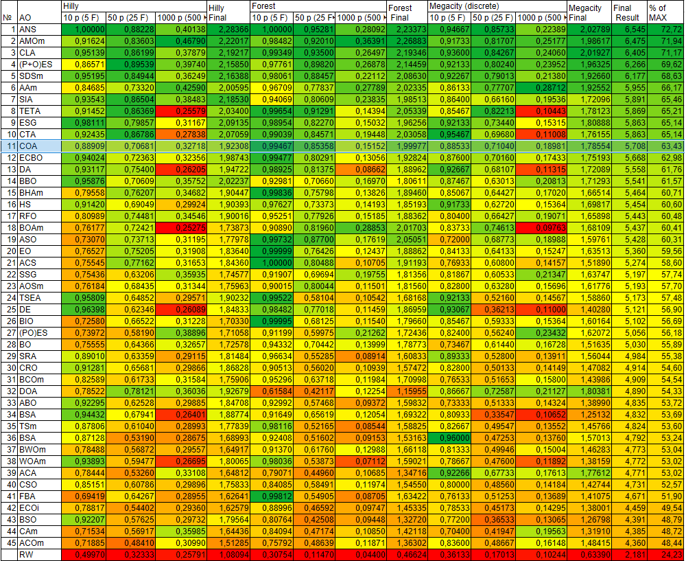
Figure 2. Color-coded ranking of algorithms based on the corresponding tests
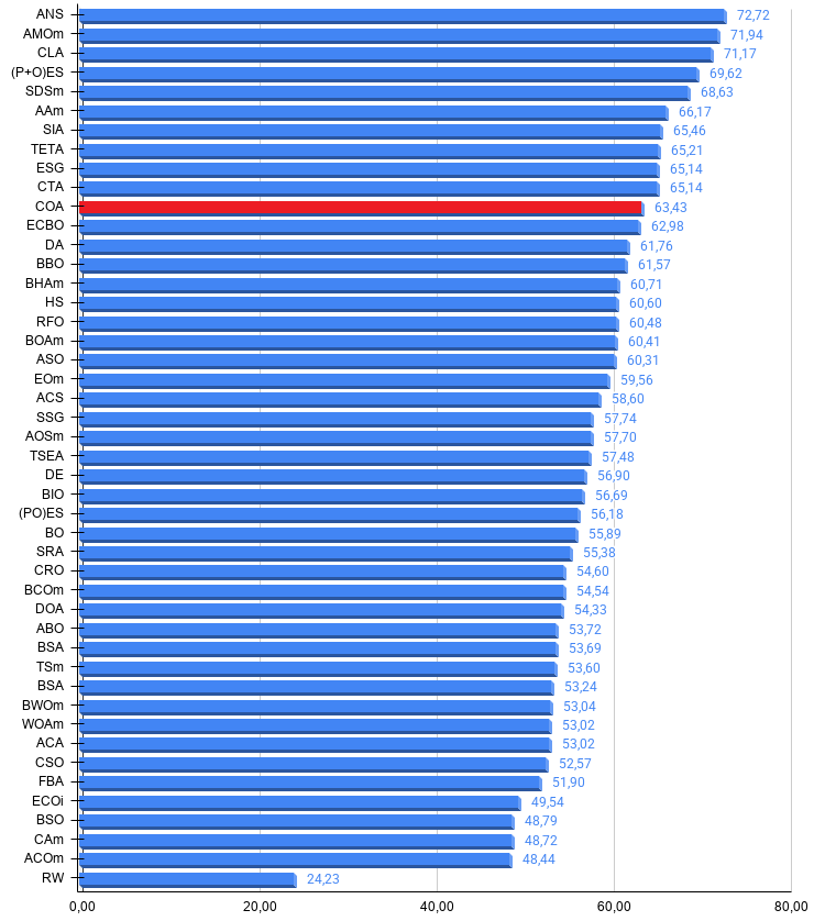
Figure 3. A histogram of the algorithm test results (on a scale from 0 to 100, with higher scores indicating better results, where 100 is the theoretical maximum); the archive contains a script for calculating the ranking table
Pros and cons of the COA algorithm:
Pros:
- A small number of external parameters.
- Good convergence.
Cons:
- With a small population, the variation in results increases.
An archive containing the latest versions of the algorithm source code is attached to the article. The author of this article does not guarantee absolute accuracy in the descriptions of canonical algorithms; many of them have been modified to improve their search capabilities. The conclusions and judgments presented in the articles are based on the results of the experiments conducted.
Software used in this article
| # | Name | Type | Description |
|---|---|---|---|
| 1 | #C_AO.mqh | Include file | Parent class for population-based optimization algorithms |
| 2 | #C_AO_enum.mqh | Include file | Enumeration of population-based optimization algorithms |
| 3 | TestFunctions.mqh | Include file | Test function library |
| 4 | TestStandFunctions.mqh | Include file | Test bench function library |
| 5 | TestStand3D.mqh | Include file | 3D visualization panel for the test bench |
| 6 | Utilities.mqh | Include file | Utility function library |
| 7 | CalculationTestResults.mqh | Include file | Script for calculating results for the comparison table |
| 8 | Test_AO_All.mq5 | Script | Unified test bench for all population-based optimization algorithms |
| 9 | Test_AO_AntiCheat | Script | Test for cheating in optimization algorithms |
| 10 | Simple use of population optimization algorithms.mq5 | Script | Simple example of using population-based optimization algorithms without visualization |
| 11 | Test_AO_COA.mq5 | Script | Test bench for COA |
Translated from Russian by MetaQuotes Ltd.
Original article: https://www.mql5.com/ru/articles/23053
Warning: All rights to these materials are reserved by MetaQuotes Ltd. Copying or reprinting of these materials in whole or in part is prohibited.
This article was written by a user of the site and reflects their personal views. MetaQuotes Ltd is not responsible for the accuracy of the information presented, nor for any consequences resulting from the use of the solutions, strategies or recommendations described.