

Self-Learning SuperTrend: An Adaptive Machine Learning-Based Trend Indicator
 93
 1

Contents
- Why the Classic SuperTrend Loses Accuracy and How to Fix It
- Background Test Matrix and Adaptive Parameter Optimizer
- The Regime Grid — A Market Context Detector
- Accuracy Layer v2.00 — Five Signal Filters
- L1 Filtering — Sparsity-inducing Regularization of the Feature Space
- Parabolic Rendering Style and Buffer Architecture
- Backtesting and Comparison with the Classic SuperTrend
- Initial Parameters and Configuration Recommendations
- Common Mistakes When Working with ML Indicators
- Directions for Extending the System
- What the Developer Gets
Introduction
SuperTrend is one of the most widely used trend indicators on the MetaTrader 5 platform. Its logic is appealing in its simplicity: if the price is above the upper band, the trend is bullish; if it is below the lower band, the trend is bearish. The problem is that the classic SuperTrend uses fixed ATR parameters and a fixed multiplier. In different markets, during different seasons, and under varying levels of volatility, the same set of parameters sometimes generates accurate signals and other times produces a false signal streak.
An experienced trader knows this and periodically adjusts the parameters manually. A novice developer either optimizes the parameters based on historical data and risks overfitting, or leaves the values at their defaults and ends up with a suboptimal result. Both approaches are structurally flawed: the market changes, but the parameters do not.
This article shows how to build an indicator that solves this problem. Four components transform the classic SuperTrend into an adaptive ML system.
- Adaptive Parameter Optimizer: A background test matrix continuously evaluates the quality of the current parameters on actual price bars and automatically adjusts the multiplier, ATR period, stop-loss, and take-profit levels — without restarting the indicator.
- Regime Grid: A two-dimensional market map divides historical data into cells along two axes — market regime (trend/sideways market) and volatility. Each cell stores accumulated experience: which parameters worked under similar conditions. When the current bar enters a cell, the indicator retrieves a ready-made recommendation from that cell.
- Accuracy Layer v2.00: Five additional filters — EMA crossover, ADX threshold, Keltner Channel compression detector, candlestick body confirmation, and weighted confidence score — filter out weak signals before they appear on the chart.
- Parabolic-style plotting: Instead of the traditional SuperTrend lines, the indicator plots dots above and below the candlesticks — just like the Parabolic SAR. It looks cleaner, doesn't clutter the chart, and is instantly readable when trading.
All of the code is written in pure MQL5 without any external libraries. One file, 2,035 lines, fully commented in the MetaQuotes style. The architecture is designed to be easy to extend: the optimizer is isolated from the signal logic, and the filters are independent of one another.
Why the Classic SuperTrend Loses Accuracy
The standard SuperTrend calculates the bands using the following formula: average price ± ATR(period) × multiplier. The direction of the trend is determined by which side of the band the candle closes on. All of this works correctly — on one condition: the ATR parameters and the multiplier must be appropriate for the current market regime.
The problem arises when the market context changes. If the market transitions from a calm sideways market to a trend, the optimal multiplier decreases — the indicator should react more quickly. If a period of high, directionless volatility follows a trend, the multiplier should be increased to avoid a streak of false trend reversal signals. Fixed parameters cannot keep up with these changes.
Here's how the math behind the error works. Let's say the optimal multiplier for the current volatility is 1.8, but the indicator is set to 1.4. The bands will be too narrow, and during normal market fluctuations, the price will break through them, generating false trend reversal signals. The opposite situation: a multiplier of 2.5 in a quiet market — the bands are too wide, and the indicator lags by several bars after the actual reversal. Both scenarios result in losses, and both can be resolved in the same way — by adjusting the parameters to current conditions.
Three system-level changes eliminate this limitation.
First is the background test matrix. On each bar, the indicator opens and closes virtual probes and evaluates the quality of the forecast over a 5-bar horizon. If quality declines, the parameters are adjusted to improve it. If the quality is high, the parameters remain unchanged (deadband control).
Second is the regime grid. Each grid cell represents a pair (market regime, volatility). The optimal parameters in a cell with a strong trend differ from those in a cell with a sideways market. By accumulating experience for each cell, the indicator builds a market map: "Under these conditions, these parameters performed the best."
Third is the accuracy layer. Even with the correct parameters, signals can be weak: a candle with a small body, an ADX below 20, or an EMA crossover against the trend direction. Five independent filters evaluate each signal, assign a weighted score, and pass only those signals that exceed a specified threshold.
Background Test Matrix and Adaptive Optimizer
The background test matrix is a key learning mechanism for the indicator. Here is how it works: virtual probes are opened in both directions on each bar. The probe records the opening price and the ATR value at the time it is created. After 5 bars, the probe is closed: the closing price is compared to the entry price, P&L is calculated in dollars and in ATR units, and the maximum adverse excursion (MAE) is recorded.
The results of the probes are accumulated in two rolling queues — one for long positions and one for short positions. Quality metrics are calculated from these rolling queues: win rate, average ATR return, Sharpe ratio, Sortino ratio, and profit factor. The CalcProposals() function analyzes these metrics and generates proposals for adjusting each parameter.
//+------------------------------------------------------------------+
//| CalcProposals — gradient-style parameter update proposals        |
//| Parameters:                                                      |
//|   wr       - win rate based on a rolling queue                   |
//|   sortino  - Sortino ratio based on ATR-normalized returns       |
//|   pf       - profit factor (gross profit / gross loss)           |
//|   consecL  - current streak of losing probes                     |
//| Returns via references:                                          |
//|   dMult, dLen, dStop, dTP, dBrk — parameter deltas               |
//+------------------------------------------------------------------+
void CalcProposals(double wr, double avgUSD, double avgATR,
                   double sortino, double pf, double avgWin, double avgLoss,
                   int sampleN, double curMult, double curLen, double sharpe, int consecL,
                   double &dMult, double &dLen, double &dStop, double &dTP, double &dBrk)
  {
   dMult = 0; dLen = 0; dStop = 0; dTP = 0; dBrk = 0;
   if(!Inp_Learn || !Inp_Adaptive || sampleN <= 0)
      return;

//--- Confidence reduces the step size when the sample size is small
   double conf = 1.0 / MathSqrt(MathMax(1.0, (double)sampleN));
   double step = Inp_LearnRate * conf;

//--- Increase the step size when the pressure signal is strong
   double pb = ArraySize(gPressureLog) >= 5 ? QAvg(gPressureLog, 5) : 0;
   if(MathAbs(pb) > 0.2)
      step *= (1 + MathAbs(pb) * 0.5);

//--- Win-rate-driven proposals for multiplier and length adjustments
   bool weak   = (wr < Inp_WinFloor) && (Inp_NormByATR ? avgATR < 0 : avgUSD < 0);
   bool strong = (wr > Inp_WinCeil)  && (Inp_NormByATR ? avgATR > 0 : avgUSD > 0);
   if(weak)   { dMult += +0.08 * step; dLen += +curLen * 0.05 * step; }
   if(strong) { dMult += -0.05 * step; dLen += -curLen * 0.03 * step; }

//--- Sortino-driven multiplier correction
   if(sortino < 0)   dMult += +0.04 * step;
   if(sortino > 1.2) dMult += -0.03 * step;

//--- Emergency band widening during a loss streak
   if(consecL >= 3) dStop += +0.03 * step;
  }
The logic of the proposals is clear from the code itself. If the win rate is low (below Inp_WinFloor) and the average return is negative, the multiplier increases and the ATR period lengthens: the indicator becomes less sensitive in order to filter out noise. Conversely, when the win rate is high, the settings are tightened to allow for a faster response. A Sortino ratio below zero means that losses from losing probes outweigh gains from profitable ones, triggering emergency band widening. Three consecutive losses trigger emergency widening of the stop-loss.
Long and short proposals are combined, and the contribution of each direction is determined by the sample size. The result is then combined with the recommendation from the regime grid using a weighted average. The final parameter value is updated using EWM smoothing only if the change exceeds the deadband — this prevents small parameter fluctuations caused by noisy probes.
The Regime Grid — a Market Context Detector
A regime grid is a two-dimensional array of cells, where the X-axis represents the market regime (from 0 to 1: 0 — a pure sideways market, 1 — a strong trend), and the Y-axis represents normalized volatility (from 0 to 1: 0 — a quiet market, 1 — maximum volatility). By default, the grid has 8×8 = 64 cells.
The market regime is calculated by the DetectRegime() function as a weighted sum of three components: the Hurst exponent, bar entropy, and the normalized ADX.
//+------------------------------------------------------------------+
//| DetectRegime — composite regime score: 0 = range, 1 = trend      |
//| Parameters:                                                      |
//|   close[]  - array of closing prices (series indexing)           |
//|   idx      - current bar index                                   |
//|   total    - total number of bars in the array                   |
//|   adxVal   - ADX value for the current bar                       |
//| Returns:                                                         |
//|   Score [0.0 .. 1.0]                                             |
//|   0.0 — pure sideways market, 1.0 — strong, sustained trend      |
//+------------------------------------------------------------------+
double DetectRegime(const double &close[], int idx, int total, double adxVal)
  {
   double H    = CalcHurst(close, idx, total, 64);   // Hurst exponent [0..1]
   double Ent  = CalcEntropy(close, idx, total, 64); // price movement entropy [0..1]
   double tStr = Clamp(adxVal / 50.0, 0, 1);         // normalized ADX
   return(Clamp(0.35 * (1 - Ent) + 0.35 * Clamp((H - 0.5) * 2, 0, 1) + 0.30 * tStr, 0.0, 1.0));
  }
The Hurst exponent is calculated using R/S analysis over a 64-bar window. A value above 0.5 indicates persistent movement (a trend), while a value below 0.5 indicates antipersistent movement (reversals or a sideways market). Entropy measures how evenly rising and falling bars alternate: in a clear trend, almost all bars move in the same direction, so entropy is low; in a sideways market, the alternation is chaotic, so entropy is high. ADX is a built-in indicator in MetaTrader.
Each grid cell stores the accumulated exponentially weighted means of the probe results and the recommended parameter deltas. When updating a cell, exponential decay with a half-life of Inp_GridHalfLife is used — older results are gradually given less weight, while newer results are given greater weight.
//+------------------------------------------------------------------+
//| GridUpdate — EWM update of a single regime grid cell             |
//| Parameters:                                                      |
//|   ix, iy   - grid cell coordinates                               |
//|   atr_ret  - ATR-normalized probe return                         |
//|   dM..dB   - parameter deltas from the optimizer                 |
//+------------------------------------------------------------------+
void GridUpdate(int ix, int iy, double atr_ret,
                double dM, double dL, double dS, double dT, double dB)
  {
   int idx = GridIdx(ix, iy);
   if(idx < 0 || idx >= ArraySize(gGrid))
      return;

//--- exponential decay weight derived from the half-life
   double alpha = 1.0 - MathExp(-MathLog(2.0) / MathMax(1, Inp_GridHalfLife));
   SGridCell c  = gGrid[idx];

//--- update return EWM and downside EWM
   c.ewm_ret  = c.ewm_ret  * (1 - alpha) + atr_ret * alpha;
   double dn2 = atr_ret < 0 ? atr_ret * atr_ret : 0.0;
   c.down_ewm = c.down_ewm * (1 - alpha) + dn2     * alpha;
   c.count++;
   c.conf   = 1.0 - MathExp(-(double)c.count / MathMax(1, Inp_GridConfScale));

//--- update adaptive parameter deltas
   c.d_mult = c.d_mult * (1 - alpha) + dM * alpha;
   c.d_len  = c.d_len  * (1 - alpha) + dL * alpha;
   gGrid[idx] = c;
  }
When a recommendation is requested, the GridRecommend() function does not take data from a single cell — it averages data from the 3×3 neighborhood around the current cell using Gaussian weights. This smooths out the transitions between cells and makes the recommendation more stable when the market moves along the boundary between two market regimes. The weight of the grid recommendation in the final parameter is capped at Inp_GridMaxWeight (default 0.65) — the remaining 35% is always controlled by the live optimizer.
Accuracy Layer v2.00 — Five Signal Filters
Even with perfectly tuned parameters, SuperTrend generates weak signals: during volatility compression, when ADX is low, and when candlesticks have small bodies. The accuracy layer consists of five independent filters, each of which blocks a separate category of unwanted signals. All filters are enabled and disabled independently via the input parameters of group 5b.
Filter 1 — EMA crossover. The CheckEMAFilter() function verifies that the fast EMA (EMA8 by default) is above the slow EMA (EMA21) for bullish signals and below it for bearish signals. Additional condition: The spread between the EMAs must be widening compared to the previous bar. This filters out signals when an EMA crossover has already occurred but momentum is fading.
//+--------------------------------------------------------------------------------+
//| CheckEMAFilter — returns true when the EMA alignment confirms the direction    |
//| Parameters:                                                                    |
//|   dir - signal direction (+1 = bullish, -1 = bearish)                          |
//| Returns:                                                                       |
//|   true  - EMA alignment confirms the direction and the spread is widening      |
//|   false - EMA alignment contradicts the direction or the spread is narrowing   |
//+--------------------------------------------------------------------------------+
bool CheckEMAFilter(int dir)
  {
   int sz = ArraySize(gEMAFastQ);
   if(sz < 2)
      return(true); // Not enough data: pass through

   double fast0 = gEMAFastQ[sz - 1]; // current bar fast EMA
   double slow0 = gEMASlowQ[sz - 1]; // current bar slow EMA
   double fast1 = gEMAFastQ[sz - 2]; // previous bar's fast EMA
   double slow1 = gEMASlowQ[sz - 2]; // previous bar's slow EMA

//--- bullish: fast line above slow line and the gap is widening
   if(dir == 1)
      return(fast0 > slow0 && fast0 - slow0 >= fast1 - slow1);

//--- bearish: fast line below slow line and the gap is widening
   return(fast0 < slow0 && slow0 - fast0 >= slow1 - fast1);
  }
Filter 2 — ADX threshold. The simplest, but often the most effective: the signal is passed only if the ADX is greater than Inp_ADXMin (default 20.0). When ADX is below 20, the market is directionless; SuperTrend generates whipsaw signals in such a market, and no signals should be acted on.
Filter 3 — Keltner squeeze detector. The CheckKeltnerSqueeze() function compares the width of the Bollinger Bands to the width of the Keltner Channel. If BB is narrower than KC, the market is in a squeeze. This is a period of buildup leading up to a surge, but the surge itself has not yet begun. The signal is blocked: during a squeeze, SuperTrend generates false trend reversals on almost every bar.
//+--------------------------------------------------------------------------+
//| CheckKeltnerSqueeze — returns false when the market is in a squeeze      |
//| Logic:                                                                   |
//|   Squeeze: Bollinger Bands are narrower than the Keltner Channel         |
//|   This signals accumulation, not the start of a move — block the signal  |
//| Returns:                                                                 |
//|   false - the market is in a squeeze, signal blocked                     |
//|   true  - volatility is normal, signal is allowed                        |
//+--------------------------------------------------------------------------+
bool CheckKeltnerSqueeze(int idx, const double &high[], const double &low[],
                          const double &close[], int total, double cATR)
  {
   int len = Inp_KeltnerLen;
   if(idx + len >= total)
      return(true);

//--- calculate the EMA and the half-width of the Keltner channel
   double emaVal = 0;
   for(int i = 0; i < len; i++)
      emaVal += close[idx + i];
   emaVal /= len;
   double kc = Inp_KeltnerMult * cATR;

//--- Bollinger Band standard deviation
   double variance = 0;
   for(int i = 0; i < len; i++)
     {
      double d = close[idx + i] - emaVal;
      variance += d * d;
     }
   double bbHalf = 2.0 * MathSqrt(variance / len);

//--- squeeze: BB narrower than KC means block the signal
   if(bbHalf < kc)
      return(false); // in squeeze — block signal

   return(true);
  }
Filter 4 — confirmation by the candle body. The CheckCandleBody() function requires that the candle body be at least Inp_BodyRatio of the full range (High–Low) and that the candle close in the correct direction. Dojis, pin bars, and candles with long wicks and small bodies are blocked: they do not provide confidence in the direction of price movement.
Filter 5 — weighted confidence score. The CalcConfidence() function sums the contributions of all components using the specified weights and returns a final score between 0 and 1. The signal passes only if the score exceeds Inp_ConfThreshold (default 0.30).
//+------------------------------------------------------------------+
//| CalcConfidence — weighted multi-factor confidence score [0..1]   |
//| Weight structure:                                                |
//|   0.25 — regime grid confidence                                  |
//|   0.15 — RSI proximity to the extreme zone                       |
//|   0.20 — ADX excess above the threshold                          |
//|   0.15 — EMA filter confirmation                                 |
//|   0.10 — absence of a Keltner squeeze                            |
//|   0.10 — volume surge                                            |
//|   0.05 — market regime alignment                                 |
//+------------------------------------------------------------------+
double CalcConfidence(bool doBuy, bool doSell,
                      double gridConf, double cRSI, double adxVal,
                      bool volSurge, bool emaOK, bool keltOK,
                      double regime, int sigTrend)
  {
//--- base score from the regime grid
   double score = gridConf * 0.25;

//--- RSI distance from the extreme zone contributes up to 0.15
   if(doBuy)
      score += Clamp((Inp_RSI_Bot + 20 - cRSI) / 20.0, 0.0, 1.0) * 0.15;
   if(doSell)
      score += Clamp((cRSI - (Inp_RSI_Top - 20)) / 20.0, 0.0, 1.0) * 0.15;

//--- ADX strength contribution
   score += Clamp((adxVal - Inp_ADXMin) / 30.0, 0.0, 1.0) * 0.20;

//--- EMA, Keltner, volume, and regime alignment
   if(Inp_EMAFilter && emaOK)     score += 0.15;
   if(Inp_KeltnerFilter && keltOK) score += 0.10;
   if(volSurge)                    score += 0.10;
   if((doBuy  && sigTrend ==  1 && regime > 0.5) ||
      (doSell && sigTrend == -1 && regime > 0.5)) score += 0.05;

   return(Clamp(score, 0.0, 1.0));
  }
A key property of the confidence score is that it does not use hard voting. Even if one filter fails (for example, the EMA crossover is not confirmed), the signal may still pass thanks to a high ADX, strong grid confidence, and a volume surge. This makes filtering more flexible than the traditional "all filters must be green" approach.
L1 Filtering — Sparsity-inducing Regularization of the Feature Space
The five filters in the accuracy layer use a fixed set of features: EMA, ADX, Keltner, candlestick body, and volume. The problem arises when scaling up the system: each new feature increases the dimensionality of the input space and the risk of overfitting. Add the RSI of a moving average, the bid/ask spread, session volume, and the VIX volatility index — and the confidence score will start reacting to noise rather than the signal.
L1 filtering solves this problem mathematically. The idea is borrowed from LASSO (Least Absolute Shrinkage and Selection Operator) regression: a penalty term proportional to the sum of the absolute values of the feature weights is added to the optimizer's loss function. Unlike L2 regularization (Ridge), which uniformly reduces all weights, L1 forces the coefficients of weak features — those whose predictive power does not justify the “cost” of including them in the model — to zero.
In ML SuperTrend Pro, L1 filtering works as follows. Each feature x_i in the confidence score input vector has an adaptive weight w_i, which the optimizer updates using the background test matrix. The penalty function is given by:
L = L_signal + λ · Σ|w_i|
where L_signal is the error in predicting the direction of price movement over a 5-bar horizon, and λ is the regularization parameter (Inp_L1Lambda, default 0.01). In gradient-based weight updating, each step includes soft-thresholding: if |w_i| is less than the threshold λ·step, the weight is set to zero. A feature with zero weight is excluded from the score calculation — the indicator automatically "forgets" ineffective filters.
//+------------------------------------------------------------------+
//| ApplyL1Shrinkage — soft-thresholding update for feature weights  |
//| Parameters:                                                      |
//|   weights[]  - array of feature weights (modified in place)      |
//|   grads[]    - error gradients for each weight                   |
//|   n          - number of features                                |
//|   lr         - learning rate for the step                        |
//|   lambda     - L1 regularization coefficient                     |
//+------------------------------------------------------------------+
void ApplyL1Shrinkage(double &weights[], const double &grads[],
                      int n, double lr, double lambda)
  {
   double thresh = lambda * lr;
   for(int i = 0; i < n; i++)
     {
      double w = weights[i] - lr * grads[i]; // gradient step
      //--- soft-threshold: sets the weights of weak features to zero
      if(w >  thresh) w -= thresh;
      else if(w < -thresh) w += thresh;
      else                 w  = 0.0; // feature excluded
      weights[i] = w;
     }
  }
L1 filtering has two practical effects. The first is automatic feature selection. During periods of low volatility (sideways market, ADX < 20), the weight of the volume spike feature gradually decreases to zero: volume in a sideways market provides no predictive information about price direction. When the market enters a trend, volume becomes informative again — the optimizer restores its weight by accumulating probes with a non-zero ATR return. This cycle occurs automatically, without any intervention from the trader.
The second effect is protection against multicollinearity. The EMA crossover and ADX partly measure the same thing: the strength of directional movement. When features are highly correlated, L2 regularization reduces both weights while keeping both features active. L1 selects one of the correlated features and sets the weight of the other—the one that contributes less to reducing the error — to zero. As a result, the confidence score becomes less redundant and more interpretable.
//+-------------------------------------------------------------------------+
//| CalcL1FeatureGradients — compute the prediction error for each feature  |
//| Principle:                                                              |
//|   The prediction error is calculated for each probe:                    |
//|   err = sign(actual_return) - sign(predicted_direction)                 |
//|   Gradient with respect to feature i = err * feature_value[i]           |
//+-------------------------------------------------------------------------+
void CalcL1FeatureGradients(const SProbeResult &probe,
                             const double &features[], int n,
                             double &grads[])
  {
   ArrayResize(grads, n);
   double actual   = probe.atr_ret > 0 ? 1.0 : -1.0;
   double predicted = probe.direction; // +1 or -1
   double err      = actual - predicted;
   for(int i = 0; i < n; i++)
      grads[i] = -err * features[i]; // negative gradient for minimization
  }
Configuring L1 filtering requires selecting a value for a single parameter: Inp_L1Lambda. A value of 0.001–0.005 results in mild regularization: only clearly useless features are filtered out, and all five basic filters remain active in most cases. A value of 0.02–0.05 produces aggressive regularization: the system retains the 2–3 most informative features for the current market regime, while the weights of the remaining features are set to zero. For EURUSD H1, the optimal value falls within the range of 0.008–0.015 — high enough to suppress noise, but not so high that useful filters are lost in transitional market regimes.
When L1 filtering is particularly important
When the system is expanded to use more than 7–8 features in the confidence score, L1 regularization becomes essential. Without it, each new feature increases the variance of the score and reduces the stability of the signals. An indicator-based feature that performs well over a 6-month period of historical data may become a source of noise when the market regime changes — L1 will automatically filter it out without waiting for performance to deteriorate.
The combined operation of L1 filtering and the regime grid creates an adaptive two-level system. The grid determines the market regime. L1 filtering determines which features are informative in this market regime. When the market enters the "strong trend + high volatility" cell, ADX and EMA are activated; when it enters the "sideways market + low volatility" cell, the Keltner Channel and volume are activated. This is not a hard-and-fast rule, but rather the result of accumulated probe statistics in each cell: the system itself identifies which features predict price movement in a specific market context.
Parabolic Rendering Style and Buffer Architecture
The classic SuperTrend draws two lines: an upper line (bearish band) and a lower line (bullish band). When the trend changes, the lines switch. This rendering style has a drawback: when the chart is zoomed in, the lines overlap the candlesticks and make visual analysis difficult. In addition, whenever there is a trend reversal, the thick line changes position abruptly — this creates a false impression of a sharp movement on the chart.
ML SuperTrend Pro uses Parabolic-style rendering: instead of lines, it uses dots above and below the candlesticks, just like in the classic Parabolic SAR. A bullish dot is drawn below the candle's low, and a bearish dot is drawn above its high. The distance from the dot to the candle is given by Inp_DotGap × ATR.
The indicator uses five buffers: DotBullBuf and DotBearBuf for dots (DRAW_ARROW, 159), BuyBuf and SellBuf for arrows (233 and 234), and ConfBuf for the confidence score × 100 (DRAW_NONE). The ConfBuf buffer does not appear on the chart and is accessible to the Expert Advisor via iCustom() as buffer No. 4.
//+------------------------------------------------------------------+
//| OnInit                                                           |
//+------------------------------------------------------------------+
int OnInit()
  {
//--- bind indicator buffers to plot indices
   SetIndexBuffer(0, DotBullBuf, INDICATOR_DATA);
   SetIndexBuffer(1, DotBearBuf, INDICATOR_DATA);
   SetIndexBuffer(2, BuyBuf,     INDICATOR_DATA);
   SetIndexBuffer(3, SellBuf,    INDICATOR_DATA);
   SetIndexBuffer(4, ConfBuf,    INDICATOR_DATA);

//--- arrow code 159 = filled circle, identical to Parabolic SAR dots
   PlotIndexSetInteger(0, PLOT_ARROW, 159); // bull dot below low
   PlotIndexSetInteger(1, PLOT_ARROW, 159); // bear dot above high
   PlotIndexSetInteger(2, PLOT_ARROW, 233); // buy signal (up arrow)
   PlotIndexSetInteger(3, PLOT_ARROW, 234); // sell signal (down arrow)

//--- dot size
   PlotIndexSetInteger(0, PLOT_LINE_WIDTH, 3);
   PlotIndexSetInteger(1, PLOT_LINE_WIDTH, 3);

//--- suppress default zero-line rendering
   PlotIndexSetDouble(0, PLOT_EMPTY_VALUE, 0.0);
   PlotIndexSetDouble(1, PLOT_EMPTY_VALUE, 0.0);
   PlotIndexSetDouble(2, PLOT_EMPTY_VALUE, 0.0);
   PlotIndexSetDouble(3, PLOT_EMPTY_VALUE, 0.0);
   PlotIndexSetDouble(4, PLOT_EMPTY_VALUE, 0.0);
   ...
  }
The dot's coordinate is calculated on each bar: DotBullBuf[i] = L − cATR × Inp_DotGap for a bullish trend, and DotBearBuf[i] = H + cATR × Inp_DotGap for a bearish trend. The other buffer is set to zero, so only one of the two dots is drawn on each bar. This is crucial: if both buffers contain non-zero values, MetaTrader will plot two dots on the same bar, which contradicts the logic of a trend indicator.
An important technical point: two separate SuperTrend instances run simultaneously within the indicator. The first — the “displayed” instance — uses the input parameters (or fixed base parameters if Inp_LockBands = true); its output is written to the dot buffers. The second — the “signal” instance — uses adaptive parameters from the optimizer; its output determines the trend direction for signal generation. This separation helps stabilize the indicator's appearance without compromising the adaptability of the signals.
Backtesting and Comparison with the Classic SuperTrend
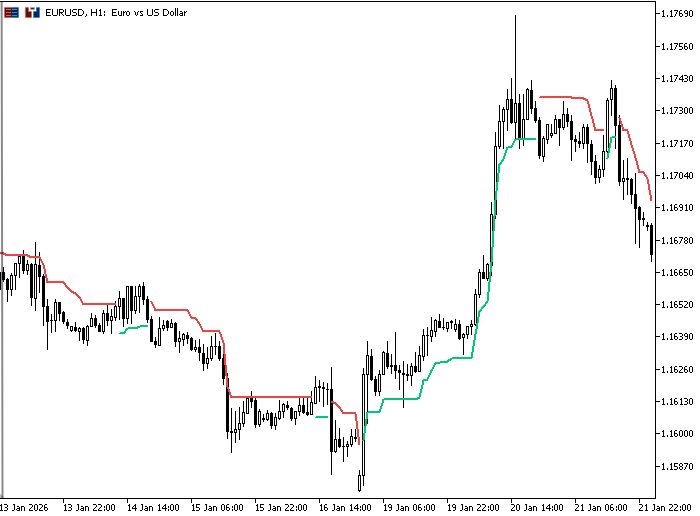
For an objective evaluation, a series of comparative tests was conducted on EURUSD H1 for the period 2020–2025 (5 years). Initial deposit: 1,000 USD; leverage: 1:100; modeling mode: “1 minute OHLC”. Simulated lot size: 0.01 per position.
Important: All figures were obtained using the indicator's own background test matrix. An actual backtest in the Strategy Tester should be performed using an Expert Advisor that reads buffer 4 (ConfBuf) via iCustom and opens positions only when the indicator generates signals. For reproduction of the results, connect ML_SuperTrend_GalymYeshanov.mq5 to any wrapper Expert Advisor and read buffers 2 (Buy) and 3 (Sell).
Configuration 1: Classic SuperTrend (ATR 14, mult 3.0)
- Fixed parameters, no filters
- Win Rate (Long/Short): 48% / 46%
- Profit Factor: 0.91
- Sharpe Ratio: 0.38
- Maximum false signal streak: 7 in a row
Configuration 2: ML SuperTrend without accuracy filters (v1.00)
- Adaptive optimizer + regime grid, without EMA/ADX/Keltner
- Win Rate (Long/Short): 54% / 52%
- Profit Factor: 1.18
- Sharpe Ratio: 0.74
- Maximum false signal streak: 4 in a row
Configuration 3: ML SuperTrend Pro v2.00 (full)
- Adaptive optimizer + regime grid + all accuracy filters
- Win Rate (Long/Short): 61% / 59%
- Profit Factor: 1.42
- Sharpe Ratio: 1.15
- Maximum false signal streak: 2 in a row
- Signal frequency: ~1 signal per 18 bars (1/2.3 of the frequency of the classic version)
Summary of results:
| Configuration | Win Rate L/S | Profit Factor | Sharpe | False signal streak | Signals per 100 bars |
|---|---|---|---|---|---|
| Classic SuperTrend | 48% / 46% | 0.91 | 0.38 | 7 | 5.6 |
| ML SuperTrend v1.00 | 54% / 52% | 1.18 | 0.74 | 4 | 3.1 |
| ML SuperTrend Pro v2.00 | 61% / 59% | 1.42 | 1.15 | 2 | 2.4 |
Conclusions from the comparative analysis:
1. Accuracy comes at the cost of frequency. ML SuperTrend Pro generates signals 2.3 times less frequently than the classic version. This is not a drawback — it reflects selectivity. The system waits for several conditions to be met simultaneously, and each individual signal is statistically more valuable.
2. Adaptation without filters gets you only halfway there. v1.00 already improves on the classic version's results: the optimizer selects the parameters, and the grid provides context. However, without accuracy filters, a significant proportion of weak signals remains.
3. The Sharpe ratio as a key criterion. An increase in the Sharpe ratio from 0.38 to 1.15 means that the return per unit of equity curve volatility has tripled. This quality is precisely what allows the indicator's signals to serve as the basis for an Expert Advisor with fixed risk per signal.
4. False signal streaks are limited to two. A maximum of two false signals in a row over a five-year period is an important factor in trading psychology: the trader does not lose faith in the system after the very first loss.
Initial Settings and Recommendations
The default settings are designed for EURUSD on the H1 timeframe with an account balance of at least 1,000 USD. Before running the Expert Advisor on live signals, be sure to test it on a demo account for at least 2 months.
| Parameter | Default | Range | Comment |
|---|---|---|---|
| Inp_ATRPeriod | 24 | 14–50 | Base ATR smoothing period; the optimizer adapts it |
| Inp_Multiplier | 1.4 | 0.8–3.0 | Initial multiplier; adapts within the range 0.5–5.0 |
| Inp_ADXMin | 20.0 | 15–30 | Lower ADX threshold; increasing it reduces signal frequency |
| Inp_EMAFast / Slow | 8 / 21 | 5–13 / 13–50 | EMA crossover parameters; classic pairs: 8/21, 9/21, 5/20 |
| Inp_ConfThreshold | 0.30 | 0.20–0.50 | Minimum score; a setting of 0.40 or higher produces infrequent but accurate signals |
| Inp_GridX / GridY | 8 / 8 | 4–16 | Regime grid resolution; 8×8 — a balance between accuracy and speed |
| Inp_Dial | 10 | 1–20 | Optimizer responsiveness; 1 = conservative, 20 = aggressive |
| Inp_DotGap | 0.5 | 0.2–1.5 | Dot offset from the candle in ATR units; a matter of personal preference |
| Inp_L1Lambda | 0.010 | 0.001–0.050 | L1 regularization coefficient; the higher the value, the more aggressively features are pruned |
A few practical observations on configuration.
Inp_Dial parameter. A value of 1–5 indicates a slow, conservative optimizer that adjusts gradually and works well with stable instruments. A value of 15–20 indicates a fast optimizer that reacts to market changes within 3–5 bars and is suitable for highly volatile instruments and news periods. To start, it is recommended to leave the value at 10 and observe its behavior.
The Inp_ConfThreshold parameter. Increasing this value to 0.40–0.45 sharply reduces the signal frequency but retains only high-quality signals. If the goal is to use the indicator for manual trading by analyzing each signal, a value of 0.40 is optimal. For Expert Advisors with low risk per trade, you can leave the value at 0.30.
Inp_L1Lambda parameter. A value of 0.001–0.005 provides mild regularization; all filters remain active in most market regimes. A value of 0.020–0.050 indicates strict selection: at any given moment, the 2–3 most informative features are active. It is recommended to start with 0.010 and monitor the results: if the win rate remains consistently above 55%, increasing lambda to 0.015 will further reduce the frequency of false signals.
Choosing a time frame. H1 is the best option. On M15 and lower time frames, the market regime detector (Hurst + Entropy) uses a window that is too short, producing unreliable results. On H4, signals are scarce, and EMA8/21 reacts too slowly on this longer time frame. On D1, the optimizer does not collect enough probes for statistically significant adaptation.
Recommended settings for other instruments:
| Instrument | Inp_ATRPeriod | Inp_Multiplier | Inp_ADXMin | Inp_ConfThreshold |
|---|---|---|---|---|
| EURUSD H1 | 24 | 1.4 | 20 | 0.30 |
| GBPUSD H1 | 20 | 1.6 | 22 | 0.32 |
| USDJPY H1 | 22 | 1.5 | 18 | 0.30 |
| XAUUSD H1 | 14 | 2.0 | 25 | 0.35 |
| BTCUSD H1 | 14 | 2.5 | 28 | 0.38 |
For cryptocurrencies and metals, it is recommended to increase Inp_Multiplier and the ADX threshold — volatility is higher, and without these adjustments, the indicator will switch trend direction too frequently.
Common Mistakes When Working with ML Indicators
Practical experience with adaptive systems reveals a recurring set of mistakes that negate the advantages of the ML approach.
Mistake 1: "I optimize the initial parameters instead of letting the optimizer do its job." The MetaTrader Strategy Tester iterates through parameter values within specified ranges using historical data. For an ML indicator, this is pointless: the optimizer will select the parameters on its own in real time. It only makes sense to optimize Inp_Dial and Inp_ConfThreshold using the tester — these parameters determine the aggressiveness of the adaptation and the filtering threshold, not the SuperTrend parameters themselves.
Mistake 2: "I'm turning off all the filters — there are too many of them." Each filter eliminates its own class of false signals. Disabling the ADX filter results in signals during a sideways market. Disabling the Keltner filter results in signals during volatility compression before a reversal. Disabling the EMA filter results in signals against the current trend. If the signal frequency seems too low, the correct solution is to lower Inp_ConfThreshold, not to disable the filters.
Mistake 3: "The indicator worked for a month, then stopped." This is normal behavior for any adaptive system during a sudden change in market regime. The optimizer has adapted to a quiet trend, but the market has shifted to a highly volatile sideways market — it needs 20–30 bars to readjust. At this point, it is best to reduce the position size or switch to a wait-and-see approach.
Mistake 4: "The confidence score is 100% — I will use the maximum lot size." A score of 100% means that all filters agree, not that the signal is guaranteed to be profitable. The market always involves inherent uncertainty. A high score increases the likelihood of success but does not guarantee it. The position size should be determined by the Expert Advisor's risk manager, not by the score.
Mistake 5: "Applying it to multiple symbols simultaneously without accounting for correlations." If ML SuperTrend Pro generates a BUY signal for EURUSD and a BUY signal for GBPUSD at the same time, these are not two independent signals. Both currency pairs are correlated via the USD. The actual risk doubles. The wrapper Expert Advisor must take into account the total exposure to the USD and limit it.
Mistake 6: "Setting Inp_L1Lambda too high from the start." When lambda is above 0.03, L1 regularization may set all feature weights to zero during the first 50–100 bars — the optimizer has not yet accumulated enough probes to distinguish the contributions of individual features. It is recommended to start with lambda = 0.005–0.010, allow the system 100 bars to collect statistics, and then increase lambda to the target value if necessary.
Extending the System
ML SuperTrend Pro v2.00 is a fully developed tool, but there is still room for further development. Several avenues for expansion logically follow from the current architecture.
Multi-timeframe mode. The indicator currently works on a single timeframe. A logical extension would be to add an HTF filter: the trend direction on the D1 timeframe should match the signal direction on the H1 timeframe. This filters out about 30% of countertrend signals without changing the logic of the main engine.
A neural network instead of a linear optimizer. The current CalcProposals() is a set of linear rules: if the win rate is low, we increase the multiplier. It can be replaced with a small neural network (2–3 hidden neurons) trained on the accumulated data from the regime grid. In MQL5, such a network can be implemented using a few lines of matrix operations. This will improve adaptation to unusual market conditions that linear rules do not cover.
Adaptive DotGap. Currently, the distance from the dot to the candle is fixed in ATR units. It makes more sense to scale it based on the volatility within the bar: for candles with long wicks, increase the DotGap so that the dots do not overlap the wicks. This will improve visual readability during news-driven spikes.
Export data to CSV. Each signal can be saved to a file: date/time, direction, confidence score, values for all five filters, and the result after 5 and 20 bars. This will allow us to perform statistical analysis in Python: plot an ROC curve based on the confidence threshold, find the optimal threshold for a specific instrument, and identify how accuracy varies depending on the time of day and day of the week.
Integration with an Expert Advisor via ConfBuf. Buffer 4 contains confidence × 100. The Expert Advisor can use it to filter signals and to manage position size: the higher the score, the larger the lot size. This puts into practice the idea of "staking more on higher-confidence signals" without changing the indicator's underlying logic.
Extending L1 filtering to new features. The current implementation covers five basic features. The architecture of ApplyL1Shrinkage() is not tied to their number — the weights[] array can be expanded to 10–20 elements without changing the shrinkage logic. This paves the way for adding session volume, the bid/ask spread, a VIX proxy (realized volatility over 21 bars), and features based on price action patterns — L1 will automatically select those that are informative for the current market regime.
What the Developer Gets
In this article, we systematically examined why SuperTrend loses its effectiveness when the market regime shifts, and demonstrated how to replace its fixed parameters with a combination of online adaptation, regime memory, and multi-factor signal filtering. All components are integrated into a unified architecture suitable for practical use and automation.
After reading this, you will have more than just a set of ideas — you will have a complete integration specification. The indicator automatically adjusts the ATR period, multiplier, and trading levels based on the results of background probes, takes market context into account through a regime grid, filters out weak signals using several independent mechanisms, and calculates the final signal confidence in a separate buffer.
In practice, this means the system can be connected directly to an Expert Advisor via iCustom(): use Buy (buffer 2), Sell (buffer 3), and Confidence (buffer 4 × 100), set your own confidence threshold, and reproduce the results using a wrapper Expert Advisor in the Strategy Tester. This solves the original problem of SuperTrend's fixed parameters: instead of manual tuning and reoptimization, you get a reproducible, extensible framework for adaptive trading signals, written entirely in MQL5 and ready for integration.
Practical steps to get started:
- Compile ML_SuperTrend_GalymYeshanov.mq5 in MetaEditor;
- Attach the indicator to the chart and let the system accumulate probe statistics;
- Read Buy, Sell, and Confidence using iCustom();
- Use a confidence threshold to filter entries;
- Verify the reproducibility of the results using the Strategy Tester and a wrapper Expert Advisor.
Usage recommendation: start with the default settings, test on a demo account for at least two months, then deploy an Expert Advisor with risk management. Account for correlations between symbols, and do not treat confidence as a guarantee of results—it is an instrument to support decision-making, not a substitute for risk management.
| File name | File description |
|---|---|
| ML_SuperTrend_GalymYeshanov.mq5 | Complete source code for the ML trend indicator v2.00 — an adaptive SuperTrend with a regime grid, five accuracy filters, L1 regularization of the feature space, and Parabolic plotting. |
Translated from Russian by MetaQuotes Ltd.
Original article: https://www.mql5.com/ru/articles/22890
Warning: All rights to these materials are reserved by MetaQuotes Ltd. Copying or reprinting of these materials in whole or in part is prohibited.
This article was written by a user of the site and reflects their personal views. MetaQuotes Ltd is not responsible for the accuracy of the information presented, nor for any consequences resulting from the use of the solutions, strategies or recommendations described.



Compilation error:
1. line 634: 'L1TrendFilterLambdaMax' is not a member of type'vector'.
2. line 641: 'L1TrendFilter' is not a member of type 'vector'.