

Corona Virus Optimization (CVO) Algorithm
 56
 1

Contents
Introduction
The number of nature-inspired optimization algorithms is growing every year, and nearly every new study promises attractive plots showing rapid convergence. For a trader looking to optimize the parameters of their trading system, it is becoming increasingly difficult to distinguish a truly powerful tool from a mediocre one presented in a favorable light on easy, low-dimensional problems. Corona Virus Optimization (CVO) is based on a model of coronavirus spread: infected individuals transmit symptoms to susceptible individuals, the infected population grows or is renewed after another success, and the force of infection controls the size of the search step. It is a fresh idea, and the original paper reports strong results — but how will the algorithm perform on a fair benchmark shared by all algorithms, without cherry-picking convenient test functions?
In this article, I walk through the implementation of CVO: from the original formulas to working code in the standard C_AO test harness. I explain how the dynamic population works, the meaning of R0 and the force of infection I/N, and the necessary departures from the original paper. The most important of these is coordinate-wise perturbation, which prevents the algorithm from exploiting the diagonal symmetry of the test functions. Next comes a run on the standard test suite (Hilly, Forest, and Megacity in 10, 50, and 1,000 dimensions) and, more importantly than the results themselves, an analysis of why a strictly faithful implementation performed only as well as a random walk and what exactly lifts it above that level.
By the end, you will have not only a ready-to-use, framework-compatible implementation of CVO and an honest assessment of its position in the overall rankings. You will also gain something more broadly applicable — an understanding of why following a published formula to the letter sometimes yields poor results, and how a single change can make the algorithm effective again.
Implementation of the Algorithm
CVO is based on the SIR (Susceptible–Infectious–Recovered) epidemiological model. The population is divided into susceptible individuals, infected individuals, and recovered/deceased individuals. An infected individual comes into contact with susceptible individuals and transmits symptoms to them; if a susceptible individual's immunity is weaker than the carrier's, they become ill and join the infected population. Over time, the number of infected individuals grows according to the basic reproduction number R0, while the force of infection scales the intensity of transmission. Carriers with strong immunity recover or die and leave the population.
The authors’ analogy to optimization is as follows: the patient is the solution, the patient’s symptoms are the variables of the problem, and the level of immunity is the value of the fitness function. The key — and at first counterintuitive — point: weak immunity = a better solution. The weaker a patient's immune system, the closer they are to the optimum; therefore, GlobalBest stores the patient with the weakest immunity over the entire run, while LocalBest stores the patient with the weakest immunity in the current iteration. This is a minimization problem: the lower the immunity value, the better the solution.
Other notation: basePop — initial number of infected individuals, nPop — population ceiling, Iters — number of iterations (recurrences of the pandemic), R0 — the number of susceptible individuals infected by a single carrier, pop — the entire infected population, newPop — newly infected individuals in the current iteration, ρ — the contact rate (assumed to be 1).
Three equations. Rate of symptom transmission (Eq. 1):
τ = ρ · φ;
where ρ is the contact rate, and φ is the probability of symptom transmission.
Force of infection (Eq. 2):
λ(I) = τ · (I / N);
where I is the number of infected individuals and N is the total population. In other words, the higher the proportion of infected individuals, the greater the force of infection and the larger the perturbation.
For continuous problems, φ is drawn from the standard normal distribution via the Box–Müller transformation (Eq. 3):
Z = √(−2·ln U₁) · cos(2π·U₂), where U₁ and U₂ are drawn from the uniform distribution U(0,1)
Combining these expressions, carrier x generates a susceptible individual by changing each symptom independently:
xₙₒв[j] = x[j] + ρ · Zⱼ · (I / N); clamped to [LB, UB]
Important: a separate Zⱼ is sampled for each coordinate — the author explicitly states that each symptom changes randomly and independently, even though they are all transmitted simultaneously.
Infection rule (selection). Immunity (fitness) is calculated for each susceptible individual. If a susceptible individual's immunity is weaker than the carrier's immunity (f(xₙₒв) < f(x) — that is, the solution is better for the optimization problem), the individual becomes infected and is added to newPop. Susceptible individuals with strong immune systems have "followed the protocols" and are not added to the new population. At the same time, LocalBest for the current iteration is tracked.
Population dynamics (end of iteration):
- if LocalBest < GlobalBest (a new global best has been found) — GlobalBest is updated, and the entire pop is replaced with newPop;
- otherwise, newPop is appended to pop (the population grows);
- if |pop| > nPop, pop is sorted in ascending order of immunity, and the best nPop individuals are retained (the rest have recovered or died).
Pseudocode for the algorithm:
ρ = 1
pop ← basePop random candidate solutions in [LB, UB]; evaluate
GlobalBest ← best of pop
for iter = 1..Iters:
    newPop ← ∅;  LocalBest ← worst
    for each x carrier from pop:
        repeat R0 times:
            for each j variable:
                Z ← BoxMuller()
                xₙₒв[j] ← clamp( x[j] + ρ·Z·(|newPop|/nPop), LB, UB )
            f ← fitness(xₙₒв)
            if f < fitness(x):            # weaker than the carrier → becomes infected
                newPop ← newPop ∪ {xₙₒв}
            if f < LocalBest: LocalBest ← xₙₒв
    if LocalBest < GlobalBest:
        GlobalBest ← LocalBest;  pop ← newPop      # replacement
    otherwise:
        pop ← pop ∪ newPop                         # growth
    if |pop| > nPop:
        sort pop in ascending fitness order; leave best nPop
return GlobalBest
A simple example (1 variable). A carrier is at x = 2.0, with ρ = 1; at an early iteration, few individuals are infected, so let I/N = 0.1. With R0 = 3, it generates three susceptible individuals with Z = {0.8, −1.5, 0.2}: the steps are ρ·Z·(I/N) = {0.08, −0.15, 0.02}, giving new points {2.08, 1.85, 2.02}. The steps are tiny, so the search is local. As the pandemic spreads and I/N approaches 1, the same mechanism produces steps on the order of Z, so the search becomes broader.
This leads to two properties of the canonical algorithm worth keeping in mind (we will discuss them later): the step increases as the population fills up — in contrast to classical annealing, where it decreases; and replacing pop with newPop when an improvement is found resets the population and shrinks the step again. In other words, stagnation broadens the search, while success narrows it.
From minimization to maximization. Everything described above follows the original formulation: the weakest immunity corresponds to the lowest function value, which is also the best. Selection retains individuals with weaker immune systems — that is, patients with lower function values.
The C_AO framework, into which we are porting the algorithm, works the other way around — it maximizes. All test functions in the series are normalized so that a higher score is better; the global best fB is the maximum, and the base class and the entire ranking are based on the principle that "higher is better." For CVO to fit into the series and be fairly compared with the other algorithms, it must use the same maximization convention.
Therefore, when porting the code, we do not change the algorithm itself—we reverse the direction of all comparisons so that "better" always means "a higher f." The correspondence is as follows:
- weaker immunity = better (min) → higher f = better (max);
- infection: previously f(susceptible individual) < f(carrier) → now f(susceptible individual) >= f(carrier);
- best-value update: previously LocalBest < GlobalBest → now LocalBest > GlobalBest;
- Pool pruning: It used to be sorted in ascending order, selecting the smallest values → it is now sorted in descending order, selecting the largest values.
The mechanics remain unchanged: a dynamic pool, R0-based spread, "infected if no worse than the carrier," replacement/growth/pruning, and step growth based on the proportion of infected individuals. Only the comparison operator changes. Thus, the comparisons in the code below will be reversed relative to those described in the article, as expected: we seek a maximum where the original sought a minimum.
Implementation in C_AO. Canonical CVO uses a dynamic population: pop grows or is replaced, and each iteration generates |pop| · R0 new patients — a variable count. The contract for the C_AO test harness is strict: For each epoch, the test harness evaluates exactly ArraySize(a) = popSize agents — it calls Moving(), calculates a[i].f using CalcFunc, calls Revision(), and repeats this process epochCount = NumbTestFuncRuns / popSize times. The function evaluation budget per epoch is fixed. These two models — a dynamic population and a fixed budget — must be reconciled.
Solution: popSize is not the CVO population, but rather the budget of susceptible individuals per epoch. On each pass, the test harness evaluates popSize candidates — susceptible individuals generated by carriers. The infection pool itself is maintained as a separate internal state, inf[]; it survives the overwriting of the a[] slots and expands or contracts according to the CVO rules. So, in total, FE = popSize · epochCount ≈ NumbTestFuncRuns, just like for all algorithms in the series, making for a fair comparison.
Each individual in the pool is represented by a structure: its symptoms (coordinates) and immunity (fitness) are stored together, following the S_AO_Agent pattern.
//+------------------------------------------------------------------+
//|                            Structure                             |
//+------------------------------------------------------------------+
struct S_CVO_Patient
 {
  double             c [];
  double             f;
 };
The full class declaration is as follows, including parameters with safeguards and pool fields:
//+------------------------------------------------------------------+
//|                             Class                                |
//+------------------------------------------------------------------+
class C_AO_CVO : public C_AO
 {
public:
                    ~C_AO_CVO() {}
                     C_AO_CVO()
   {
    ao_name = "CVO";
    ao_desc = "Corona Virus Optimization";
    ao_link = "https://www.mql5.com/en/articles/22887";

    popSize = 50;     // FE budget per epoch (= candidates per pass)
    nPop    = 200;    // maximum infected population
    basePop = 5;      // initial infected population
    R0      = 5;      // susceptible individuals (offspring) per carrier
    rho     = 0.1;    // contact rate: overall scale factor for λ

    ArrayResize(params, 5);
    params [0].name = "popSize";
    params [0].val = popSize;
    params [1].name = "nPop";
    params [1].val = nPop;
    params [2].name = "basePop";
    params [2].val = basePop;
    params [3].name = "R0";
    params [3].val = R0;
    params [4].name = "rho";
    params [4].val = rho;
   }

  void               SetParams()
   {
    popSize = (int)params [0].val;
    nPop    = (int)params [1].val;
    basePop = (int)params [2].val;
    R0      = (int)params [3].val;
    rho     =      params [4].val;

    //--- safeguards
    if(popSize < 1)
      popSize = 1;
    if(nPop    < 1)
      nPop    = 1;
    if(R0      < 1)
      R0      = 1;
    if(rho   < 0.0)
      rho     = 0.0;
    if(basePop < 1)
      basePop = 1;
    if(basePop > popSize)
      basePop = popSize; // the pool is seeded from the first batch
    if(basePop > nPop)
      basePop = nPop;
   }

  bool               Init(const double &rangeMinP  [],
                          const double &rangeMaxP  [],
                          const double &rangeStepP [],
                          const int     epochsP = 0);

  void               Moving();
  void               Revision();

  //--- visible parameters
  int                nPop;       // maximum infected population
  int                basePop;    // initial infected population
  int                R0;         // offspring per carrier
  double             rho;        // scale factor for λ

private:
  //--- infection pool (array of structures: coordinates and fitness combined)
  S_CVO_Patient      inf [];        // [nPop]
  int                infCount;      // current pool size (<= nPop)

  //--- mapping a candidate slot to a carrier
  int                parentOf [];   // [popSize]

  //--- temporary rebuild pool
  S_CVO_Patient      tmp [];        // [nPop + popSize]

  //--- standard normal distribution (Box–Muller), Eq. 3
  double             Gauss();
  //--- index sort by descending f
  void               ArgSortDesc(const double &f [], int &idx [], const int count);
 };
Mapping slots to carriers. In the canonical formulation, each carrier infects R0 susceptible individuals. For a fixed budget, this is mapped as follows: slot k is generated by carrier p = (k / R0) % infCount, meaning that R0 consecutive slots share a single carrier. If the pool is larger than popSize/R0, only the first ceil(popSize/R0) carriers reproduce — and since the pool is sorted in descending order of immunity, these are the best ones. If the pool is smaller, the modulo operation wraps the index around, and the carriers are reused. The result is an elitist projection of the "each carrier infects R0 susceptible individuals" rule onto a fixed epoch budget.
Init sets the initial random coordinates for each agent and allocates a pool and a buffer once:
//+------------------------------------------------------------------+
//|                              Init                                |
//+------------------------------------------------------------------+
bool C_AO_CVO::Init(const double &rangeMinP  [],
                    const double &rangeMaxP  [],
                    const double &rangeStepP [],
                    const int     epochsP = 0)
 {
  if(!StandardInit(rangeMinP, rangeMaxP, rangeStepP))
    return false;

//--- initial random batch in cP[] (to be evaluated on the first pass)
  for(int i = 0; i < popSize; i++)
    for(int c = 0; c < coords; c++)
      a [i].cP [c] = u.RNDfromCI(rangeMin [c], rangeMax [c]);

//--- infected pool and temporary pool (arrays of structures)
  ArrayResize(inf, nPop);
  for(int i = 0; i < nPop; i++)
    ArrayResize(inf [i].c, coords);

  ArrayResize(tmp, nPop + popSize);
  for(int i = 0; i < nPop + popSize; i++)
    ArrayResize(tmp [i].c, coords);

  ArrayResize(parentOf, popSize);
  infCount = 0;

  return true;
 }
During a normal pass, Moving generates popSize susceptible individuals, each coordinate by coordinate using the article's formula (Eq. 1·3). The step here is absolute, following the article to the letter — this is the version for the first faithful run; in the diagnostics section, we will replace just the line defining v:
//+------------------------------------------------------------------+
//|                            Moving                                |
//+------------------------------------------------------------------+
void C_AO_CVO::Moving()
 {
//--- first pass: cP -> c
  if(!revision)
   {
    for(int i = 0; i < popSize; i++)
      for(int c = 0; c < coords; c++)
        a [i].c [c] = u.SeInDiSp(a [i].cP [c], rangeMin [c], rangeMax [c], rangeStep [c]);
    return;
   }

//--- generate candidate susceptible individuals
  for(int k = 0; k < popSize; k++)
   {
    int denom = infCount > 0 ? infCount : 1; // protection against %0
    int p = (k / R0) % denom;          // the carrier for this slot
    parentOf [k] = p;

    for(int c = 0; c < coords; c++)
     {
      double phi  = Gauss();                                   // Eq. 3, [D1] separate for each coordinate
      double frac = (double)(infCount + k) / (double)nPop;     // I/N, Eq. 1*Eq. 2, [D3]
      if(frac > 1.0)
        frac = 1.0;
      double lam  = rho * phi * frac;        // absolute step, EXACTLY as specified in the article (Eq. 1*2*3)
      double v    = inf [p].c [c] + lam;
      a [k].c [c] = u.SeInDiSp(v, rangeMin [c], rangeMax [c], rangeStep [c]);
     }
   }
 }
Revision handles all the end-of-iteration operations of the canonical algorithm: updating the best solutions, seeding the pool on the first pass, selecting infected individuals, and rebuilding the population. Since the test harness maximizes, all comparisons are reversed relative to the article: an individual whose immunity is no worse than the carrier's ( >= ) becomes infected, and the best individuals are sorted in descending order:
//--- accepted susceptible individuals: immunity no better than the carrier's -> infected
//    (read inf[p].f BEFORE the pool is overwritten—there is no overlap.)
  for(int k = 0; k < popSize; k++)
   {
    int p = parentOf [k];
    if(MathIsValidNumber(a [k].f) && a [k].f >= inf [p].f)
     {
      ArrayCopy(tmp [cnt].c, a [k].c, 0, 0, coords);
      tmp [cnt].f = a [k].f;
      cnt++;
     }
   }
Next comes the replacement/growth decision and truncation, exactly as in the canonical algorithm, but adapted for maximization: if the global best improves, the pool is replaced with newly infected individuals; otherwise, accepted susceptible individuals are appended to it. If the pool exceeds its capacity, it is sorted in descending order of fitness and truncated to the best nPop individuals.
Gauss — a normal variate generated using the Box–Muller transform (Eq. 3). Converts two uniformly distributed numbers from (0, 1) into a standard normal variate; called separately for each coordinate when generating a susceptible individual:
//+------------------------------------------------------------------+
//|              Gauss — standard normal variate (Box–Muller)        |
//+------------------------------------------------------------------+
double C_AO_CVO::Gauss()
 {
  double u1 = u.RNDfromCI(0.0, 1.0);
  double u2 = u.RNDfromCI(0.0, 1.0);
  if(u1 < 1e-15)
    u1 = 1e-15;                       // Protection against ln(0)
  return MathSqrt(-2.0 * MathLog(u1)) * MathCos(2.0 * M_PI * u2);
 }
ArgSortDesc — index order by descending f. It is needed in two places (seeding and truncation). To avoid having to pass around structures, we sort not the pool itself, but a flat array of fitness values, obtaining an index order that we then use to build the result:
//+------------------------------------------------------------------+
//|     ArgSortDesc — index order by descending f                    |
//+------------------------------------------------------------------+
void C_AO_CVO::ArgSortDesc(const double &f [], int &idx [], const int count)
 {
  for(int i = 0; i < count; i++)
    idx [i] = i;

  for(int i = 0; i < count - 1; i++)
   {
    int b = i;
    for(int j = i + 1; j < count; j++)
      if(f [idx [j]] > f [idx [b]])
        b = j;
    if(b != i)
     {
      int t = idx [i];
      idx [i] = idx [b];
      idx [b] = t;
     }
   }
 }
This is a selection sort with O(count²) complexity, but count does not exceed nPop + popSize, and the sort is called once per epoch. The overhead is negligible compared with function evaluations, while the code remains extremely clear.
Test Results
We run the standard test suite used in this series: the Hilly, Forest, and Megacity functions with 10, 50, and 1,000 variables, a budget of 10,000 function evaluations, and 10 repeats each. The final score is a normalized fraction of the maximum. The step is absolute, exactly as described in the paper, with a contact rate ρ = 1, as specified by the authors. Best unmodified configuration (popSize=50, nPop=100, basePop=20, R0=10):
CVO|Corona Virus Optimization|50.0|100.0|20.0|10.0|1.0|
=============================
5 Hilly's; Func runs: 10000; result: 0.5811428685355893
25 Hilly's; Func runs: 10000; result: 0.3689998607642066
500 Hilly's; Func runs: 10000; result: 0.26725319445074575
=============================
5 Forest's; Func runs: 10000; result: 0.4021701300516501
25 Forest's; Func runs: 10000; result: 0.1679713459276718
500 Forest's; Func runs: 10000; result: 0.05216720027056517
=============================
5 Megacity's; Func runs: 10000; result: 0.4613333333333333
25 Megacity's; Func runs: 10000; result: 0.21520000000000006
500 Megacity's; Func runs: 10000; result: 0.11194666666666767
=============================
All score: 2.62818 (29.20%)
29.20%. This performance is close to that of a random walk — on tests where the stronger algorithms in the series score over fifty percent. A distinctive pattern is also evident: with 10 variables, the results are still decent (0.58 on Hilly), but as the number of variables increases, performance drops rapidly — with 1,000 variables, Forest drops to 0.05, which is essentially noise. The algorithm handles high dimensionality very poorly.
Before blaming the algorithm, you need to make sure it is calculating correctly and is not broken. The check is to test its sensitivity to parameters. With basePop=10 and R0=5 fixed, we vary the contact rate: ρ = 0.001 → 18.40%; ρ = 0.1 → 28.91%; ρ = 10
→ 24.93%.The response is smooth and meaningful: when ρ is very small, the step is nearly zero and the search stalls (18%); when ρ is large, the step becomes erratic and the search approaches a random search (25%); the optimum lies somewhere in the range ρ ≈ 0.1…1. It reacts similarly to basePop and R0 (the best values are basePop=20 and R0=10). If the logic were broken, the results would be uniformly meaningless regardless of the parameter settings. Since there is a clear optimum and a response to parameter tuning, the mechanism is working and the calculations are correct. The ~29% limit is not a bug in the implementation, but a property of the method itself in this context.
Diagnosis and Correction. Let's return to the step formula in its exact form:
λ = ρ · φ · (I / N), xₙₒв[j] = x[j] + λ
The perturbation here is absolute, expressed in raw coordinate units. When ρ = 1 and φ is drawn from a standard normal distribution, the perturbation's magnitude is on the order of one (two or three in the tails), multiplied by the proportion of infected individuals, which ranges from zero to one. In other words, a typical step is a shift of about one or two units along an axis, regardless of which axis it is.
That's where the problem lies. The step size is not tied to the width of the search region, and the benchmark functions operate over different ranges. Roughly speaking: if the axis spans, say, 200 units, then a step of about one unit represents half a percent of the range; the algorithm barely moves — it just creeps along in place. If the axis spans only a couple of units, the same step covers half the entire range, producing wild jumps and a purely random search. The same λ produces tiny steps on one function and chaos on another. This explains the results from the previous section: with 10 variables, it barely works, but with 1,000, performance collapses to the noise level, because a fixed, small absolute step cannot cover such a huge volume.
This hypothesis is easy to test: if it's a matter of scale, then mapping the step size to the range width should fix the problem. And indeed it does.
A common-sense adjustment. We make the step a fraction of each coordinate's range — just one line in Moving:
// Before (absolute step, following the article to the letter):
double v = inf [p].c [c] + lam;

// After (a fraction of the coordinate's range):
double v = inf [p].c [c] + lam * (rangeMax [c] - rangeMin [c]);
Now λ represents not an absolute distance along an axis, but a fraction of its width, with the same meaning across all functions and coordinates. The scale invariance that was missing.
But this requires retuning the magnitude. With range-scaling, the original ρ = 1 results in a step across the entire range — exactly the kind of chaos we just described (incidentally, this explains why an early attempt to scale with ρ = 1 devolved into a random search). Therefore, ρ = 0.1: with a full pool, the step size is ~0.1·φ·range, that is, on the order of 5–10% of the axis width — a reasonable value for refinement. At the same time, the pool and seeding have been adjusted: nPop = 200 (a higher upper bound, and consequently a smaller frac = (infCount+k)/nPop → smaller step → more exploitation) and basePop = 5 (a focused start). All three parameters point in the same direction — toward a controlled step tied to the scale.
CVO|Corona Virus Optimization|50.0|200.0|5.0|5.0|0.1|
=============================
5 Hilly's; Func runs: 10000; result: 0.5946817995500855
25 Hilly's; Func runs: 10000; result: 0.36906584070682485
500 Hilly's; Func runs: 10000; result: 0.26998944552451903
=============================
5 Forest's; Func runs: 10000; result: 0.5225857394828209
25 Forest's; Func runs: 10000; result: 0.19382751005851218
500 Forest's; Func runs: 10000; result: 0.053702157009133125
=============================
5 Megacity's; Func runs: 10000; result: 0.4413333333333334
25 Megacity's; Func runs: 10000; result: 0.2424
500 Megacity's; Func runs: 10000; result: 0.11301333333333437
=============================
All score: 2.80060 (31.12%)
Have we strayed too far? Formally, yes — this departs from the article's literal formulation: the article adds λ as is, while we multiply it by the range width. But this is a principled departure, not a cosmetic cheat, and here's why. First, the entire CVO structure remains intact — the dynamic pool, R0-based spread, infection “if immunity is no worse than that of the carrier,” replacement/growth, culling, and an increase in step size with the proportion of infected individuals. Only the units of perturbation have changed: absolute coordinate units → fraction of the range. Second, if the functions in the article were all of a single, moderate scale, then the authors’ absolute λ was, in fact, a reasonable proportion of their range — but in our unnormalized benchmark, this proportion must be explicitly restored. In other words, range scaling is closer to the original intent (relative step size) than the literal formula. And third, this is a standard convention throughout your entire series: all algorithms scale their step size to the range; otherwise, comparing them would be unfair.
To be honest about the magnitude of the effect: +1.9% does not turn CVO into a powerful algorithm; rather, it removes the scaling penalty that had kept it at the bottom, alongside random walk. It has now reached its true performance ceiling — the lower-middle tier. And the main generalizable lesson: when implementing any published algorithm, first check what units its step is expressed in. An absolute perturbation that looks natural on functions at the same scale misses the mark on a benchmark spanning different scales — a relative step is almost always what is needed.
The composite test with 10 variables yields 56.69%, but this is a different, easier setting (low dimensionality only), and the two figures must not be conflated — the standard 31% is used for the ranking.
CVO|Corona Virus Optimization|50.0|200.0|5.0|5.0|0.1|
=============================
Composite test: Hilly + Forest + Megacity + Peaks + Skin
Coordinates: 10; Epochs: 200; Repeats: 10
=============================
Run 1/10: 0.5598502390640241
Run 2/10: 0.46218834024270095
Run 3/10: 0.5472841349143641
Run 4/10: 0.6438002840259478
Run 5/10: 0.5363633183876485
Run 6/10: 0.6189199641420557
Run 7/10: 0.5775251324533818
Run 8/10: 0.5168167745601945
Run 9/10: 0.5741164838588073
Run 10/10: 0.6317059909142314
=============================
Average result: 0.5668570663 (56.69%)
=============================
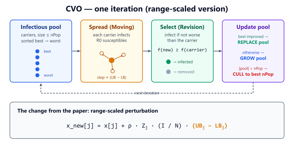
Figure 1. Diagram of the CVO algorithm
The figure shows a single iteration of the algorithm in its new, scaled version: the carrier pool generates susceptible individuals (R0 per carrier), which undergo selection (those whose immunity is at least as good as their carrier's become infected), after which the pool is updated through replacement when solutions improve, expansion during stagnation, and pruning to the best nPop individuals. In the next iteration, the cycle repeats.
The perturbation used by a carrier to generate a susceptible individual is defined by the formula shown in the illustration. The step size is determined by the force of infection
λ = ρ · φ · (I / N);
Here, ρ is the contact rate, φ = Z_j is a random number drawn from a standard normal distribution (Box–Müller transformation), independent for each coordinate j, and I / N is the proportion of infected individuals in the population. The more widespread the pandemic becomes and the higher the I/N ratio, the larger the step — the perturbation grows as the pool fills up.
The key difference from the original is the last factor (UB_j − LB_j), highlighted in orange in the diagram. In the article, the force of infection is added directly to the position, in absolute coordinate units. We multiply it by the range width of each coordinate, and the step of "so many units along the axis" becomes a fraction of the search space. This is precisely the common-sense adjustment: the same relative step behaves consistently on functions of any scale — it neither shrinks to a tiny nudge over wide ranges nor turns the search into a random one over narrow ranges. This does not affect the structure of CVO itself: only the units of the perturbation change.

CVO on the Hilly test function

CVO on the Forest test function

CVO on the Megacity test function

CVO on the Ackley test function

CVO on the Rosenbrock test function
CVO is not included in the ranking table and is presented for informational purposes only.
| cc | AO | Description | Hilly | Hilly Final | Forest | Forest Final | Megacity (discrete) | Megacity Final | Final Result | % of MAX | ||||||
| 10 p (5 F) | 50 p (25 F) | 1,000 p (500 F) | 10 p (5 F) | 50 p (25 F) | 1,000 p (500 F) | 10 p (5 F) | 50 p (25 F) | 1,000 p (500 F) | ||||||||
| 1 | ANS | across neighbourhood search | 1.00000 | 0.88228 | 0.40138 | 2.28366 | 1.00000 | 0.95281 | 0.28092 | 2.23373 | 0.94667 | 0.85733 | 0.22389 | 2.02789 | 6.545 | 72.72 |
| 2 | AMOm | animal migration optimization M | 0.91624 | 0.83603 | 0.46790 | 2.22017 | 0.98482 | 0.92010 | 0.36391 | 2.26883 | 0.91733 | 0.81707 | 0.25177 | 1.98617 | 6.475 | 71.94 |
| 3 | CLA | code lock algorithm (joo) | 0.95139 | 0.86199 | 0.37879 | 2.19217 | 0.99349 | 0.93500 | 0.26497 | 2.19346 | 0.93600 | 0.84267 | 0.24060 | 2.01927 | 6.405 | 71.17 |
| 4 | (P+O)ES | (P+O) evolution strategies | 0.86571 | 0.89539 | 0.39740 | 2.15850 | 0.97761 | 0.89820 | 0.26878 | 2.14459 | 0.92133 | 0.80240 | 0.23952 | 1.96325 | 6.266 | 69.62 |
| 5 | SDSm | stochastic diffusion search M | 0.95195 | 0.84944 | 0.36249 | 2.16388 | 0.98061 | 0.88457 | 0.22112 | 2.08630 | 0.92267 | 0.79013 | 0.21380 | 1.92660 | 6.177 | 68.63 |
| 6 | AAm | archery algorithm M | 0.84685 | 0.73320 | 0.42590 | 2.00595 | 0.96709 | 0.77837 | 0.27789 | 2.02335 | 0.86133 | 0.77707 | 0.28712 | 1.92552 | 5.955 | 66.17 |
| 7 | SIA | simulated isotropic annealing (joo) | 0.93543 | 0.86504 | 0.38483 | 2.18530 | 0.94069 | 0.80609 | 0.23835 | 1.98513 | 0.86400 | 0.66160 | 0.19536 | 1.72096 | 5.891 | 65.46 |
| 8 | TETA | time evolution travel algorithm (joo) | 0.91452 | 0.86369 | 0.25579 | 2.03400 | 0.99654 | 0.91291 | 0.14394 | 2.05339 | 0.85467 | 0.82213 | 0.10443 | 1.78123 | 5.869 | 65.21 |
| 9 | ESG | evolution of social groups (joo) | 0.98111 | 0.79857 | 0.31167 | 2.09135 | 0.98954 | 0.82270 | 0.15032 | 1.96256 | 0.92133 | 0.73440 | 0.15315 | 1.80888 | 5.863 | 65.14 |
| 10 | CTA | comet tail algorithm (joo) | 0.92435 | 0.86786 | 0.27838 | 2.07059 | 0.99039 | 0.84571 | 0.19448 | 2.03058 | 0.95467 | 0.69680 | 0.11008 | 1.76155 | 5.863 | 65.14 |
| 11 | ECBO | enhanced colliding bodies optimization | 0.94024 | 0.72363 | 0.32356 | 1.98743 | 0.99477 | 0.80291 | 0.13056 | 1.92824 | 0.87600 | 0.70160 | 0.17433 | 1.75193 | 5.668 | 62.98 |
| 12 | DA | dialectical algorithm | 0.93117 | 0.75400 | 0.26205 | 1.94722 | 0.98925 | 0.81375 | 0.08662 | 1.88962 | 0.92667 | 0.68107 | 0.11315 | 1.72089 | 5.558 | 61.76 |
| 13 | BBO | biogeography-based optimization | 0.95876 | 0.70609 | 0.35752 | 2.02237 | 0.92981 | 0.70660 | 0.16970 | 1.80611 | 0.87467 | 0.63013 | 0.20813 | 1.71293 | 5.541 | 61.57 |
| 14 | BHAm | black hole algorithm M | 0.79558 | 0.76207 | 0.34682 | 1.90447 | 0.99836 | 0.75798 | 0.13826 | 1.89460 | 0.85067 | 0.64427 | 0.17020 | 1.66514 | 5.464 | 60.71 |
| 15 | HS | harmony search | 0.91420 | 0.69049 | 0.29924 | 1.90393 | 0.97627 | 0.73373 | 0.14193 | 1.85193 | 0.91733 | 0.62720 | 0.15364 | 1.69817 | 5.454 | 60.60 |
| 16 | RFO | royal flush optimization (joo) | 0.80989 | 0.74481 | 0.34546 | 1.90016 | 0.95251 | 0.77926 | 0.15185 | 1.88362 | 0.80400 | 0.66427 | 0.19071 | 1.65898 | 5.443 | 60.48 |
| 17 | BOAm | billiards optimization algorithm M | 0.76177 | 0.72421 | 0.25275 | 1.73873 | 0.90890 | 0.81960 | 0.28853 | 2.01703 | 0.83733 | 0.74613 | 0.09763 | 1.68109 | 5.437 | 60.41 |
| 18 | ASO | anarchy society optimization | 0.73070 | 0.73713 | 0.31195 | 1.77978 | 0.99732 | 0.87700 | 0.17619 | 2.05051 | 0.72000 | 0.68773 | 0.18988 | 1.59761 | 5.428 | 60.31 |
| 19 | EOm | extremal optimization_M | 0.76527 | 0.75205 | 0.31908 | 1.83640 | 0.99999 | 0.76426 | 0.12437 | 1.88862 | 0.84133 | 0.64133 | 0.15247 | 1.63513 | 5.360 | 59.56 |
| 20 | ACS | artificial cooperative search | 0.75545 | 0.77162 | 0.31653 | 1.84360 | 1.00000 | 0.80488 | 0.10705 | 1.91193 | 0.76933 | 0.60800 | 0.14157 | 1.51890 | 5.274 | 58.60 |
| 21 | SSG | saplings sowing and growing | 0.75436 | 0.63206 | 0.35935 | 1.74577 | 0.91907 | 0.69694 | 0.19755 | 1.81356 | 0.81867 | 0.60533 | 0.21347 | 1.63747 | 5.197 | 57.74 |
| 22 | AOSm | atomic orbital search M | 0.76184 | 0.68435 | 0.31344 | 1.75963 | 0.90015 | 0.80044 | 0.11501 | 1.81560 | 0.82800 | 0.63280 | 0.15696 | 1.61776 | 5.193 | 57.70 |
| 23 | TSEA | turtle shell evolution algorithm (joo) | 0.95809 | 0.64852 | 0.29571 | 1.90232 | 0.99522 | 0.58104 | 0.10542 | 1.68168 | 0.92133 | 0.52160 | 0.14567 | 1.58860 | 5.173 | 57.48 |
| 24 | DE | differential evolution | 0.96398 | 0.62346 | 0.26089 | 1.84833 | 0.98482 | 0.77018 | 0.11459 | 1.86959 | 0.93067 | 0.36213 | 0.11000 | 1.40280 | 5.121 | 56.90 |
| 25 | BIO | blood inheritance optimization (joo) | 0.72580 | 0.66522 | 0.31228 | 1.70330 | 0.99995 | 0.68125 | 0.11540 | 1.79660 | 0.85467 | 0.59333 | 0.15364 | 1.60164 | 5.102 | 56.69 |
| 26 | (PO)ES | (PO) evolution strategies | 0.73972 | 0.58190 | 0.38896 | 1.71058 | 0.91199 | 0.59975 | 0.21262 | 1.72436 | 0.82400 | 0.56240 | 0.23432 | 1.62072 | 5.056 | 56.18 |
| 27 | BO | bonobo optimizer | 0.75555 | 0.64366 | 0.32657 | 1.72578 | 0.94332 | 0.70442 | 0.13999 | 1.78773 | 0.73467 | 0.61440 | 0.16728 | 1.51635 | 5.030 | 55.89 |
| 28 | SRA | successful restaurateur algorithm (joo) | 0.89010 | 0.63359 | 0.29115 | 1.81484 | 0.96634 | 0.55285 | 0.08914 | 1.60833 | 0.89333 | 0.52800 | 0.13911 | 1.56044 | 4.984 | 55.38 |
| 29 | CRO | chemical reaction optimisation | 0.91281 | 0.65681 | 0.29866 | 1.86828 | 0.90513 | 0.56020 | 0.10939 | 1.57472 | 0.82800 | 0.50133 | 0.14149 | 1.47082 | 4.914 | 54.60 |
| 30 | BCOm | bacterial chemotaxis optimization M | 0.82589 | 0.61733 | 0.31584 | 1.75906 | 0.95296 | 0.63718 | 0.11984 | 1.70998 | 0.76533 | 0.51653 | 0.15800 | 1.43986 | 4.909 | 54.54 |
| 31 | DOA | dream optimization algorithm | 0.78522 | 0.78121 | 0.36036 | 1.92679 | 0.61584 | 0.42117 | 0.12254 | 1.15955 | 0.86667 | 0.72587 | 0.21127 | 1.80381 | 4.890 | 54.33 |
| 32 | ABO | african buffalo optimization | 0.92295 | 0.62528 | 0.29885 | 1.84708 | 0.92992 | 0.57468 | 0.09372 | 1.59832 | 0.73333 | 0.51333 | 0.14324 | 1.38990 | 4.835 | 53.72 |
| 33 | BSA | bird swarm algorithm | 0.94432 | 0.67941 | 0.26401 | 1.88774 | 0.91649 | 0.65619 | 0.12054 | 1.69322 | 0.80933 | 0.33547 | 0.10652 | 1.25132 | 4.832 | 53.69 |
| 34 | TSm | tabu search M | 0.87806 | 0.61040 | 0.28993 | 1.77839 | 0.98116 | 0.52165 | 0.08544 | 1.58825 | 0.82667 | 0.49547 | 0.13552 | 1.45766 | 4.824 | 53.60 |
| 35 | BSA | backtracking search algorithm | 0.87128 | 0.53190 | 0.28675 | 1.68993 | 0.92408 | 0.51602 | 0.09153 | 1.53163 | 0.96000 | 0.47253 | 0.13760 | 1.57013 | 4.792 | 53.24 |
| 38 | BWOm | beluga_whale_optimization_M | 0.78488 | 0.56872 | 0.29557 | 1.64917 | 0.91370 | 0.61760 | 0.12988 | 1.66118 | 0.81333 | 0.49946 | 0.15004 | 1.46283 | 4.773 | 53.04 |
| 36 | WOAm | whale optimization algorithm M | 0.93893 | 0.59477 | 0.26695 | 1.80065 | 0.98036 | 0.53873 | 0.07112 | 1.59021 | 0.78667 | 0.47600 | 0.11892 | 1.38159 | 4.772 | 53.02 |
| 37 | ACA | andean_condor_algorithm | 0.78444 | 0.53260 | 0.33108 | 1.64812 | 0.79071 | 0.44960 | 0.10685 | 1.34716 | 0.92266 | 0.67733 | 0.17613 | 1.77612 | 4.771 | 53.02 |
| 39 | CSO | competitive swarm optimizer | 0.85151 | 0.60786 | 0.29896 | 1.75833 | 0.84085 | 0.58491 | 0.11974 | 1.54550 | 0.80000 | 0.48560 | 0.14184 | 1.42744 | 4.731 | 52.57 |
| 40 | FBA | fractal-based algorithm | 0.69419 | 0.64267 | 0.28955 | 1.62641 | 0.99812 | 0.54905 | 0.08705 | 1.63422 | 0.76133 | 0.51253 | 0.13689 | 1.41075 | 4.671 | 51.90 |
| 41 | ECOi | eco-inspired evolutionary algorithm | 0.78817 | 0.54402 | 0.29360 | 1.62579 | 0.88996 | 0.46592 | 0.09747 | 1.45335 | 0.78533 | 0.45173 | 0.14295 | 1.38001 | 4.459 | 49.54 |
| 42 | BSO | brain storm optimization | 0.92207 | 0.57625 | 0.29732 | 1.79564 | 0.80764 | 0.42508 | 0.09448 | 1.32720 | 0.77200 | 0.36533 | 0.13065 | 1.26798 | 4.391 | 48.79 |
| 43 | CAm | camel algorithm M | 0.71534 | 0.56917 | 0.35985 | 1.64436 | 0.84094 | 0.47174 | 0.10850 | 1.42118 | 0.70400 | 0.41947 | 0.19563 | 1.31910 | 4.385 | 48.72 |
| 44 | ACOm | ant colony optimization_M | 0.71885 | 0.48410 | 0.30990 | 1.51285 | 0.75792 | 0.48639 | 0.11871 | 1.36302 | 0.83600 | 0.48667 | 0.16148 | 1.48415 | 4.360 | 48.44 |
| 45 | BSO | brain storm optimization | 0.91331 | 0.55813 | 0.29705 | 1.76849 | 0.85329 | 0.44038 | 0.09447 | 1.38814 | 0.72267 | 0.32880 | 0.13325 | 1.18472 | 4.341 | 48.23 |
| CVO | corona_virus_optimization | 0.59468 | 0.36906 | 0.26998 | 1.23372 | 0.52258 | 0.19382 | 0.05370 | 0.77010 | 0.44133 | 0.24240 | 0.11301 | 0.79674 | 2.801 | 31.12 | |
| RW | random walk | 0.49970 | 0.32333 | 0.25791 | 1.08094 | 0.30754 | 0.11470 | 0.04400 | 0.46624 | 0.36133 | 0.17013 | 0.10244 | 0.63390 | 2.181 | 24.23 | |
Conclusions
CVO enters the overall ranking with its actual result — 31.12% on the standard test suite after mapping the step to the search range. The algorithm is noticeably weaker than the series leaders.
CVO does have its strengths, though. It is simple both in concept and in implementation. It incorporates an interesting adaptive mechanism: when the search stalls, the population grows, and the proportion of infected individuals drives the step up, broadening the search; when the search succeeds, pop is replaced with newly infected individuals and shrinks, reducing the step again and focusing the search. In other words, failure automatically triggers exploration, while success triggers refinement. It works in low dimensions.
The weaknesses outweigh the strengths and are clearly evident in the numbers. The main weakness is the collapse in performance at high dimensionality: with 1,000 variables, the results drop to the noise level, and no amount of step scaling can fix this because the cause runs deeper. CVO has no direct attraction to the global best: perturbations occur only around carriers, and the selection rule, "becomes infected if no worse than the carrier," provides only weak elitism. The global best is stored, but it does not draw the search toward itself. In addition, the step in the canonical version increases as the population fills up — the opposite of classical annealing, where it decays toward the end; refinement occurs only through a population reset upon improvement, rather than gradually. This is not sufficient for smooth convergence in a large space.
Now, let's get to the reason this whole thing was started — and this fulfills the promise made in the introduction. The original question was: another nature-inspired algorithm has emerged with big promises — is it worth paying attention to, and how can you tell a strong algorithm from an overhyped one? A concrete example has provided the answer: a literal, letter-for-letter implementation of CVO performs on a par with a random walk and breaks down as dimensionality increases. One change based on common sense — converting the step size from absolute units to a fraction of the coordinate range — restored the algorithm’s true performance limit, adding a couple of percent without breaking any part of it. The generalizable lesson: when implementing any algorithm, first check the units of its perturbation step; an absolute displacement, natural for functions on the same scale, misses the mark on a mixed-scale benchmark, whereas a relative step is almost always what is needed.
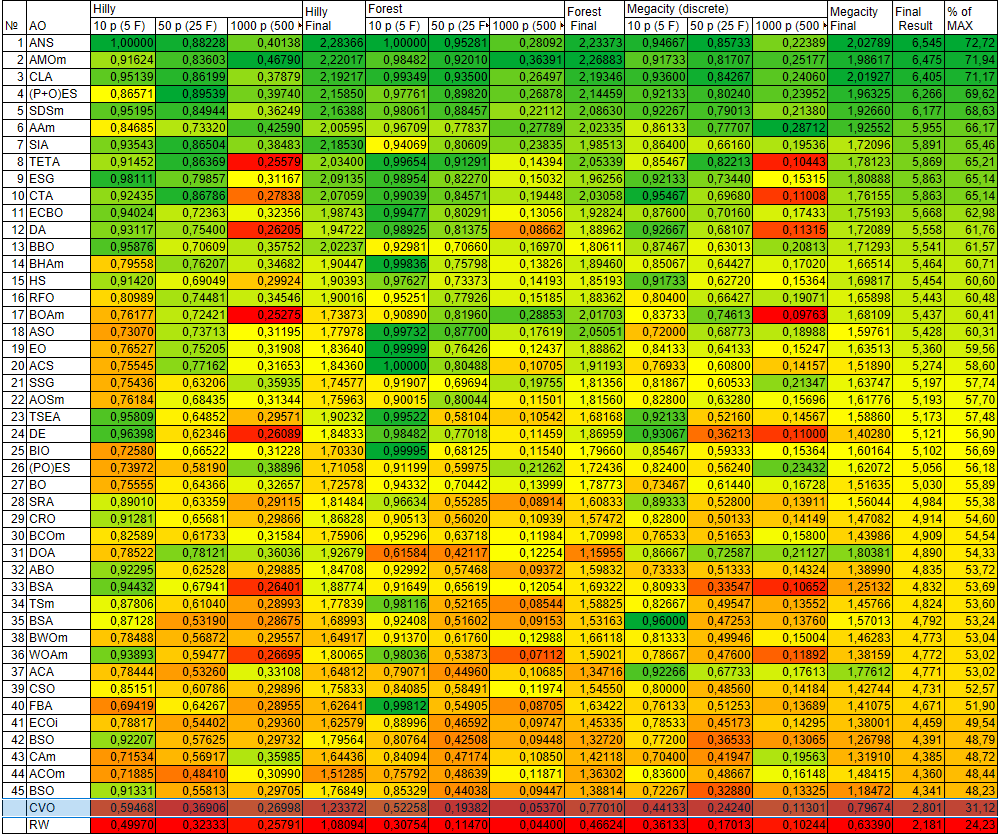
Figure 2. Color grading of the algorithms for the corresponding tests
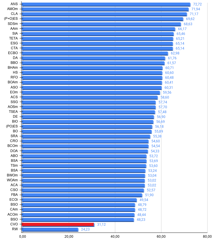
Figure 3. A histogram of the algorithm test results (on a scale from 0 to 100; the higher the score, the better, where 100 is the maximum possible theoretical result); the archive contains a script for calculating the ranking table
Pros and cons of the CVO algorithm:
Pros:
- None identified.
Cons:
- Prone to stagnation.
An archive containing the latest versions of the algorithm code is attached to the article. The author of this article is not responsible for the absolute accuracy of the descriptions of canonical algorithms; changes have been made to many of them to improve search capabilities. The conclusions and judgments presented in the articles are based on the results of the experiments conducted.
Software used in this article
| # | Name | Type | Description |
|---|---|---|---|
| 1 | #C_AO.mqh | Include file | Parent class for population-based optimization algorithms |
| 2 | #C_AO_enum.mqh | Include file | Enumeration of population-based optimization algorithms |
| 3 | TestFunctions.mqh | Include file | Test function library |
| 4 | TestStandFunctions.mqh | Include file | Library of test harness functions |
| 5 | TestStand3D.mqh | Include file | 3D visualization panel for the test harness |
| 6 | Utilities.mqh | Include file | Library of utility functions |
| 7 | CalculationTestResults.mqh | Include file | Script for calculating results for the comparison table |
| 8 | Test_AO_All.mq5 | Script | Unified test harness for all population-based optimization algorithms |
| 9 | Test_AO_AntiCheat | Script | Test for cheating in optimization algorithms |
| 10 | Simple use of population optimization algorithms.mq5 | Script | Simple example of using population-based optimization algorithms without visualization |
| 11 | Test_AO_CVO.mq5 | Script | Test harness for CVO |
Translated from Russian by MetaQuotes Ltd.
Original article: https://www.mql5.com/ru/articles/22887
Warning: All rights to these materials are reserved by MetaQuotes Ltd. Copying or reprinting of these materials in whole or in part is prohibited.
This article was written by a user of the site and reflects their personal views. MetaQuotes Ltd is not responsible for the accuracy of the information presented, nor for any consequences resulting from the use of the solutions, strategies or recommendations described.



Well done.
Have you seen the Tianji Horse Racing Optimisation?
https://link.springer.com/article/10.1007/s10462-025-11269-9
It looks interesting. Can it be replicated for MQL5?