

Estimate the Probability of Large-range Sessions (Part 1): Build and Check EURUSD Forecasts
 91
 0

Contents
- Introduction
- Define the 08:00 forecast
- Fit the model in SPSS
- Compare the 2024 forecasts
- Check how probabilities match outcomes
- Recalculate the forecasts in MetaTrader 5
- Limitations and Reproducibility
- Conclusion
Introduction
Suppose it were 8 a.m. What would your estimate be of the probability the EUR/USD pair trades a range over the next 8 hours that is significantly larger than the norm? Morning bars have stopped updating, so the highs and lows of the forthcoming bars are unknown. For example, can we say something about the range of the EUR/USD session, between 08:00 and 16:00, without knowing in which direction the session will move? H1 bars opening from 08:00 to 15:00 will be used for the analysis.
We need a way to define what we consider to be a large range. We can define large range sessions by finding the average range of the prior 20 complete and valid target windows, and increasing this value by 25%. If that average was 40 pips, we would say a large range would be anything over 50 pips.
This example shows how to fit a model in IBM SPSS Statistics and generate the model's 2024 probabilities in MetaTrader 5. The output probabilities are then compared to two historical frequency forecasts, and the average forecast loss for each of the three methods is calculated for the historical sample. The attached code allows you to conduct this type of analysis using your own EURUSD H1 data.
The 25% setting is used for illustration and is not optimized to the test case. Examples are generated using IBM SPSS Statistics 31.0.0.0 build 117 and MetaTrader 5, build 6198. To follow the examples, you will need SPSS to perform binary logistic regression, MetaTrader 5 with MetaEditor and Python 3.
Define the 08:00 forecast
| Item | Definition |
|---|---|
| Candidate dates | Monday–Friday |
| Decision time | 08:00 |
| Predictor window | Bars opening 00:00 through 07:00 |
| Target window | Bars opening 08:00 through 15:00 |
| Outcome available | 16:00 |
| Historical scale, A | Mean range of the previous 20 complete valid target windows |
| Range budget | 1.25 × A |
| Outcome, Y | For a complete valid target: 1 if its range exceeds the budget; otherwise 0 |
The range for a window is the highest high less the lowest low for the eight bars in the window. For a complete, valid target window, assign Y = 1 if its range exceeds the budget; otherwise assign Y = 0. An incomplete target has no label. The historical scale A, which excludes the current session, represents the previous 20 valid and complete target window ranges.
Each bar must have a positive and finite high, low, open and close. The high of a bar must be no less than the open or close and the low of a bar must be no greater than the open or close. All eight predictor bars must be present and closed by 08:00 and have a combined range greater than zero. Large, valid ranges are allowed, and A must be positive.
The target window must contain the eight bars and be closed by 16:00. A target window may have a zero range.
The audit log includes three flags: forecast_eligible, estimation_eligible and comparison_eligible. The forecast_eligible flag requires valid predictor inputs and history. The estimation_eligible flag also requires a complete, valid target window closed by 16:00. The comparison_eligible flag also requires 60 earlier resolved, eligible sessions for the rolling event-frequency benchmark.
| Period | Use |
|---|---|
| 2019 | Initialize the historical lookbacks |
| 2020–2023 | Estimate coefficients and training constants |
| 2024 | Evaluate the frozen model |
| 2025 | Reserved for a later article; not loaded here |
2024 cases are not included in model estimation. The coefficients, constant training frequency and calibration boundaries from 2020 to 2023 remain the same. Evaluation of history is done in chronological order. Once a 2024 target is complete and valid, its range is incorporated into the scale history for subsequent forecasts. The outcome of the event is incorporated into the rolling history only if the inputs of the forecast are also valid. Each forecast utilizes history which has been resolved earlier, and its own target is added afterward.
The exporter creates each eight-hour window using expected H1 open times. It checks the prices and closure of these windows. The current session’s features are computed prior to saving the completed target range or eligible outcome in the historical queues. The verifier reads and validates the structure of the CSV files, pairs records by session ID and recalculates features and probabilities using saved SPSS coefficients. The function and file format are described in the README.
Current session inputs are computed and written prior to updating the historical queues. If a case becomes estimation eligible, it is added to the event history. A valid and closed current target window results in its range being added to the range history, regardless of the session’s forecast eligibility.
//+------------------------------------------------------------------+
//| OnStart - forecast eligibility and history updates (excerpt)     |
//+------------------------------------------------------------------+
   double x1=0,x2=0;
   bool forecast=pre.valid && preClosed && rc==20 &&
                 SessionFeatures(pre.o,pre.h,pre.l,pre.c,a,x1,x2);
   bool eligible=forecast && target.valid && closed;
   bool comparison=eligible && ec==60;

// ...
//--- Update histories only after computing and writing today's forecast inputs.
   if(eligible)
     {
      events[epos]=ExceedsBudget(target.h-target.l,a);
      eventEnds[epos]=ending;
      epos=(epos+1)%60;
      if(ec<60)
         ec++;
     }
   if(target.valid && closed)
     {
      ranges[rpos]=target.h-target.l;
      rangeEnds[rpos]=ending;
      rpos=(rpos+1)%20;
      if(rc<20)
         rc++;
     }
The sample contains 37,315 H1 bars and 1,566 weekdays. The following table shows the distribution of the 1,295 cases by year.
| Year | Retained study observations |
|---|---|
| 2020 | 259 |
| 2021 | 260 |
| 2022 | 259 |
| 2023 | 258 |
| 2024 | 259 |
The overall workflow is summarized in Figure 1. Historical EURUSD H1 data are used to construct the morning-session predictors and the corresponding target outcomes. The logistic regression model is trained on 2020–2023 sessions, evaluated on the 2024 holdout sample, and its probability calculations are independently reproduced in MQL5.
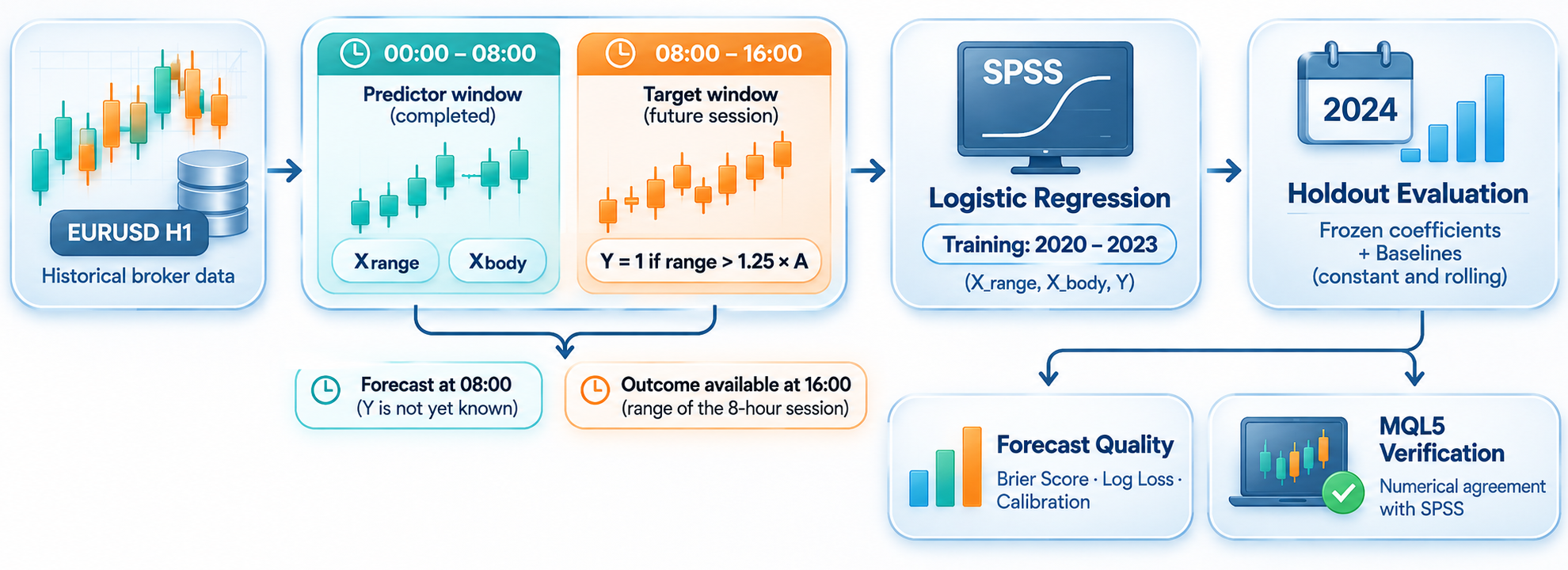
Figure 1. Overview of the EURUSD session-range probability forecasting and evaluation workflow
Fit the model in SPSS
Build the variables in SPSS
Rpre is defined as the range between the highest and the lowest values of the first eight bars of the day, which open between 00:00 and 07:00. pre_open is the open for the 0:00 bar and pre_close is the close for the 7:00 bar. The model has two inputs.
x_range = ln(1 + Rpre/A)
x_body = |pre_close − pre_open| / Rpre
x_range compares the completed morning range with A, the mean of the previous 20 valid target ranges. If the mean of the last 20 valid target ranges is constant, a larger morning range provides a larger input. The input is relative, and no expected price range is implied. x_body measures the absolute open-close move as a fraction of Rpre, from 0 to 1, ignoring direction.
SessionRisk.sps: import and predictors
The code in SessionRisk.sps first sets the working directory and captures the SPSS output. It then reads 14 session-related fields. It calculates the morning and target ranges, creates the two predictors, and defines an event if the target range exceeds its budget. Next, it identifies the training and holdout samples and calculates the smoothed rolling probability from the 60 earlier eligible outcomes. The syntax assumes the inputs are in the expected format and valid. It does not reconstruct the original H1 windows.
COMPUTE pre_range=pre_high-pre_low.
COMPUTE range_budget=1.25*prior20_mean.
COMPUTE x_range=LN(1+pre_range/prior20_mean).
COMPUTE x_body=ABS(pre_close-pre_open)/pre_range.
COMPUTE exceed=(target_high-target_low>range_budget).
COMPUTE train=(year>=2020 AND year<=2023).
EXECUTE.
Target prices determine the event label and are excluded from the predictors.
SPSS estimates the two coefficients and intercept using 2020–2023 sessions, saves the model, and calculates probabilities for the 2024 holdout cases. MQL5 uses the saved coefficients to calculate probabilities without invoking SPSS.
Training fit and saved outputs
The model-fitting block in SessionRisk.sps limits estimation to cases from 2020 to 2023. It saves SPSS model probabilities and the fitted model. The next block calculates a constant frequency baseline and bin boundaries for the training data. These values are appended to the main dataset.
LOGISTIC REGRESSION VARIABLES exceed
 /METHOD=ENTER x_range x_body
 /SELECT=train EQ 1
 /CRITERIA=ITERATE(100) BCON(1E-8) LCON(0)
 /PRINT=ITER(1)
 /SAVE=PRED(p_logit)
 /OUTFILE=MODEL('results/session_model.xml').
Do not remove the 2024 cases from the working file. The SELECT subcommand restricts fitting to train = 1, and saves the holdout cases’ probabilities.
Figure 2 shows how the cases were split: 1,036 training cases and 259 held-out cases. There were 237 training events, and the model converged in 6 iterations. Holdout cases are used to test the model against cases outside the training set.
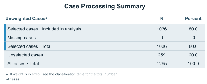
Figure 2. Case selection redrawn from SPSS output: 1,036 training cases and 259 held-out cases
The SPSS probability model is described by the equation.
p = 1 / [1 + exp(−z)]
z = −2.3346123464739601 + 3.58061255447844 × x_range − 0.84054808364295597 × x_body
On January 2, 2024, Rpre was 0.00288, and A was 0.0046325. Therefore, the budget was 0.005790625. The absolute open-close move was 0.00106, so x_range was 0.483471621 and x_body was 0.368055556. At 08:00, the model estimated that there was a 28.64% chance that the 08:00 to 16:00 range would be greater than 0.005790625. Between 08:00 and 16:00, the actual range was 0.00897. Therefore, Y equals 1. Exceedance of a threshold in a single instance does not verify the skill of a forecast model.
An intercept-only model is illustrated in Step 0 of Figure 3, and a model with two features is illustrated in Step 1. The equation represents the model in Figure 3. For the SPSS model, MQL5 uses full-precision coefficients.
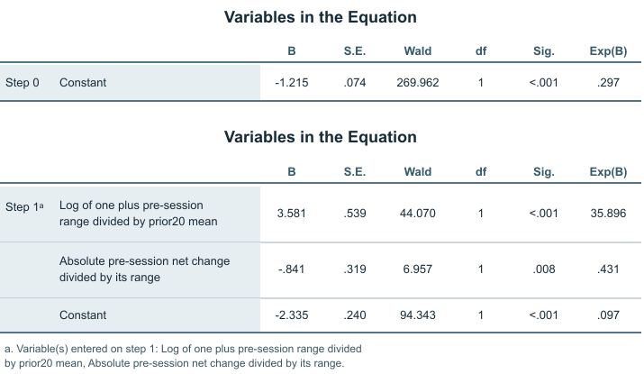
Figure 3. Coefficient estimates redrawn from SPSS output for the intercept-only model (Step 0) and two-feature model (Step 1)
The Wald statistics and Sig. values (p-values) in Figure 3 relate to the training coefficients and do not assess the statistical significance of the differences in loss in 2024.
Let’s consider the other variable as being fixed. The model’s predicted probability of exceeding the range budget rises with larger relative pre-session ranges, and falls with larger body fractions.
RiskSigmoid
RiskSigmoid converts a finite linear score z to a probability. For z >= 0, it uses 1/(1 + exp(-z)); for z < 0, it uses exp(z)/(1 + exp(z)). Both branches keep the exponential argument nonpositive to avoid overflow. The verifier checks that z is finite before calling the function.
//+------------------------------------------------------------------+
//| RiskSigmoid - convert a finite score to a probability            |
//+------------------------------------------------------------------+
double RiskSigmoid(double z)
  {
//--- Keep the exponential argument non-positive in both branches.
   if(z>=0)
      return 1.0/(1.0+MathExp(-z));
   double e=MathExp(z);
   return e/(1.0+e);
  }
Compare the 2024 forecasts
Now, how much do the morning levels help with forecasting? To answer this, we will compare the model with two other forecasts available before the session's outcome. A constant forecast, based on the training sample, indicates an event occurrence rate of 237/1036, or 22.8764%.
The other method, known as the “rolling” estimate, uses the event count over the last 60 previously resolved and eligible sessions. Adding 1 to the count and 2 to the denominator in the case of Laplace smoothing keeps the probability from being 0 or 1. Forecasts will be communicated as probabilities and will not be restricted to the values of 0 and 1.
p_constant = 237/1036 = 22.8764%
p_rolling = (1 + exceedances among the previous 60 eligible sessions) / 62
The same 2024 sessions were used to evaluate each of the three methods. Brier scores are calculated as the average of (p-Y)^2 where p is the forecast probability and Y is the case label which is 0/1. For these methods, lower log losses and Brier scores indicate lower average forecast loss on the evaluated cases.
Log loss is the mean of −[Y ln(p) + (1 − Y) ln(1 − p)], with p clipped to [1e-12, 1 − 1e-12] for this calculation only. The original session forecast probabilities are used to calculate the Brier score and evaluate calibration.
Holdout coverage and outputs
The blocks in SessionRisk.sps assess the 2024 sample by checking that the three methods produce valid predictions and losses on the same rows. In the case of an incomplete holdout sample, the syntax sets all methods' probabilities and scores to missing across the whole holdout sample.
This is done to avoid reporting comparison scores for different samples. The syntax calculates and saves coverage and aggregate statistics. It retains the three training-defined probability bins even if a bin is empty. It creates the reliability plot. The outputs are assessment of probability and not assessment of trading performance.
The results/holdout_coverage.csv file should show coverage_ok = 1, with all eight counts equal to the total number of eligible 2024 holdout cases. For any given comparison, all the forecasts and associated losses must be finite for all the cases under consideration. In the original study, all 259 cases were considered for each method. Of the 259 cases, 59 cases (22.7799%) indicated the outcome of interest.
| Forecast | Mean probability | Brier score | Log loss | Brier difference from constant |
|---|---|---|---|---|
| SPSS logistic model | 21.3786% | 0.171629 | 0.524365 | −0.004278 |
| Training frequency | 22.8764% | 0.175908 | 0.536606 | 0 |
| Rolling frequency | 23.6082% | 0.180122 | 0.548199 | +0.004215 |
The differences reported for the Brier scores are for unrounded scores. Scores reported are rounded. Subtracting rounded scores may show differences for the last digit.
During testing, the model outperformed both frequency baselines using the 259 holdout sessions and yielded lower average log losses and Brier scores. The model outperformed the constant forecast, with a Brier score difference of -0.004278. This Brier score advantage was not consistently the case, as evidenced by the second-quarter comparison shown below.
The constant forecast had a lower Brier score than the model by 0.008617 during the 65 sessions in the second quarter of 2024. These results were derived from a post hoc analysis and did not change the model or sample in question. The results illustrated variability in the sample. The comparisons were made without using the threshold of 0.5 in SPSS.
Check how probabilities match outcomes
We say that a model is “well-calibrated” if forecasts correspond with the proportion of actual occurrences.
The training forecasts determine the boundaries of the three probability groups. These boundaries are fixed for 2024. If a forecast equals a group boundary, it belongs to the next lower group. Forecasts outside the training probability range are in the lowest or highest group. Ordering rules and boundary positions used in the training set are provided in the README.
The two probability boundaries, calculated from the training data and kept fixed for the 2024 evaluation, were approximately 0.183928 and 0.234717. These boundaries divide the forecasts into three groups for comparing predicted probabilities with observed event frequencies.
| Training-defined probability group | Sessions | Events | Mean prediction | Observed frequency |
|---|---|---|---|---|
| At or below first boundary | 113 | 19 | 15.2684% | 16.8142% |
| Above first, at or below second | 72 | 20 | 20.7020% | 27.7778% |
| Above second boundary | 74 | 20 | 31.3673% | 27.0270% |
The table above shows the SPSS reliability output for the group comparison. The difference between the average forecasts and the observed frequencies is shown in Figure 4.
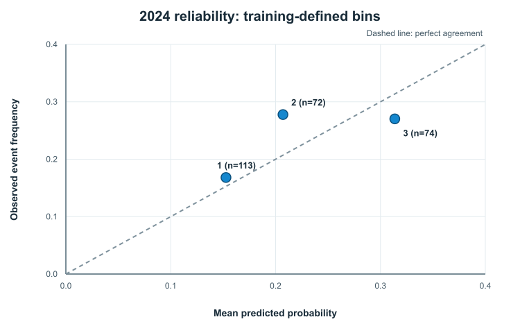
Figure 4 shows the mean predicted probability and the observed frequency of the event in 2024 for the three groups defined by the training data. The figure is created from reliability data of the study.
These differences describe calibration within the 2024 holdout sample but do not establish systematic overestimation or underestimation in future data.
In the 2024 sample, the upper group's mean forecast probability was greater than the observed event frequency, and the middle group's mean forecast was less than the observed event frequency. The upper group's observed event frequency was slightly less than the middle group's.
Recalculate the forecasts in MQL5
We will repeat the calculations in MetaTrader 5. The script VerifySessionRisk.mq5 calculates features and probabilities and compares them to the values found in SPSS.
Extract MQL5.zip into the folder opened by File > Open Data Folder in MetaTrader 5. The structure of the MQL5 folder should not change. The scripts are found in MQL5/Scripts/SessionRisk, and SessionRiskCore.mqh is found in MQL5/Include/SessionRisk.
Use MQL5/Files/SessionRisk as the working folder for SPSS and the Python commands. The CD command in SPSS should be set to this directory using forward slashes to separate directories. The data and results files are relative to this working folder. Be sure to retain your data and the results of your analysis prior to initiating a new fit or export.
Compile the scripts in MetaEditor to use them.
| macOS/Linux: | Windows: |
|---|---|
| python3 | py -3 |
- Save the results of any previous fits and create an empty directory named results.
- ExportSessionRisk.mq5: Run the compiled code on the MetaTrader 5 platform and set StudySymbol to your broker’s EURUSD symbol. FirstDate should be set to 2019-01-01 00:00:00 (inclusive) and EndExclusive to 2025-01-01 00:00:00 (exclusive) for this analysis.
- Obtain a new PASS, written by the exporter, and located in data/export_status.txt.
- Use tools/audit_export.py to check the CSV files before running the model fitting.
python3 tools/audit_export.py
- To verify your inputs, run one of these commands from the command line (terminal):
python3 tools/validate_inputs.py
If ‘PASS’ is found in results/analysis_readiness.json, you can proceed to fit the model in SPSS.
- To launch the program, open SessionRisk.sps in SPSS. In the SPSS Syntax Editor, select Run > All. Do not allow SPSS to fit the 2024 cases. Check for model convergence.
- After the model is fit, run tools/audit_results.py to check the SPSS output and create the file results/forecast_only.csv.
python3 tools/audit_results.py
- To obtain the coefficients, run one of these commands:
python3 tools/extract_coefficients.py
- VerifySessionRisk.mq5: Go to the MetaTrader 5 application and run the script. Set ExpectedRows to the total number of rows in your sessions.csv file, excluding the first/header row.
- Look for a new PASS in the file results/native_parity.txt and review results/native_predictions.csv. The permitted absolute error for features and probabilities is 1e-10.
Supporting checks
| Check | Purpose |
|---|---|
| export_status.txt | confirms completion of the export procedure and its write checks |
| export_audit.json | checks that windows and histories are reconstructed |
| analysis_readiness.json | checks that data is ready for model estimation |
| result_audit.json | verifies the saved SPSS output |
| native_parity.txt | checks arithmetic agreement with SPSS outputs |
| forecast_only_status.txt | reports the optional calculation |
A PASS is given for a specific check.
Check receipts from the current run, check if any errors are reported, and verify that audit hashes match the current input files.
Run the Python validators with assertions enabled: -O or an effective PYTHONOPTIMIZE setting is rejected.
No problems were reported when the 1,295 sessions were compared in the original study. The absolute maximum difference for a feature was 2.87e-13 and the absolute maximum difference for a probability was 5.09e-14.
Optional forecast-only calculation
The optional forecast-only calculation runs after the main comparison passes.
audit_results.py generates results/forecast_only.csv from eligible forecast windows in your export that have no valid target label. The file contains morning OHLC prices and the historical scale. If no such windows are found, a header-only file is generated. Read forecast_only_predictions.csv together with the current forecast_only_status.txt receipt. The main native_parity.txt does not validate this calculation.
July 2, 2024 illustrates the difference between forecast and evaluation eligibility. Its predictor window is complete, but three target bars are missing, so it has no event label and no loss score.
The forecast probability was 12.6749%.
Limitations and Reproducibility
The original study captured only a single snapshot of broker history for EURUSD from the MetaQuotes-Demo server, and one holdout year. All the analyses in the study used the recorded broker clock. No adjustments were made for time zones or daylight saving time. The session windows, 1.25 multiplier, 20-range scale and 60-outcome baseline were fixed, and no sensitivity analysis was performed. Other brokers, holdout years, and volatility benchmarks are unexamined. Weekday and news event effects were ignored. Stability of the parameters in varying market conditions is unknown. Therefore, the session parameters and threshold event conditions studied may not be reliably generalized.
The holdout year comparisons are descriptive. Loss difference confidence intervals and tests of significance were not reported. The calibration groups contained between 72 and 113 cases. Uncertainty intervals were not reported. As these forecasts share input data with one another, dependence and correlation between forecast errors should be considered when assessing uncertainty.
Historical replay does not show when the data would have arrived at a live process. The agreement between SPSS and MQL5 verifies the coefficient handoff and probability calculations; it does not validate predictive or trading performance. The model projects the probability of range exceedance and does not determine directionality or profit. The source code and documentation are included in the archive; however, the historical data snapshots and model outputs are not. To reproduce the results shown, the model inputs and outputs are required, as well as the versions of the software used. Full retraining of the model is not possible without SPSS. However, the broker history can be exported and checked, as can the inputs to the model. The available utilities, written in Python, do not replace SPSS for fitting the model. The complete comparison requires the SPSS coefficients and reference predictions of the study. Changes to the study period require changes to the export program, SPSS syntax, audit and validation scripts.
Conclusion
This article developed and evaluated a two-feature logistic regression model for estimating, at 08:00 broker time, the probability that EURUSD's subsequent eight-hour range would exceed 1.25 times the mean of the previous 20 valid target ranges. The model uses only information available from the completed 00:00–08:00 session and was trained on 2020–2023 data before being evaluated on 259 held-out sessions from 2024.
On the holdout sample, the model achieved lower average Brier scores and log losses than both the constant and rolling-frequency baselines. However, the improvement was modest and did not hold in every quarter. The calibration analysis also revealed differences between predicted probabilities and observed event frequencies across the three probability groups. These findings suggest that the morning-session features contain potentially useful predictive information, but do not establish stable forecasting performance beyond the examined sample.
The MQL5 implementation reproduced the SPSS-based calculations for 1,295 sessions within the predefined numerical tolerance, confirming the consistency of the coefficient transfer and probability calculations. The accompanying programs allow readers to export their own broker data, fit the specified model in SPSS, and reproduce its probabilities in MetaTrader 5. This numerical agreement should not be confused with evidence of predictive or trading profitability.
Part 2 extends the study by recalibrating the model using the already-inspected 2024 data and evaluating the updated forecasts on the reserved 2025 sample.
Attached files
| File | Location | Purpose |
|---|---|---|
| ExportSessionRisk.mq5 | MQL5/Scripts/SessionRisk | Exports historical H1 bars, session data, and a completion receipt. |
| VerifySessionRisk.mq5 | MQL5/Scripts/SessionRisk | Recalculates the predictors and probabilities and compares them with the SPSS results. |
| SessionRiskCore.mqh | MQL5/Include/SessionRisk | Includes the price checks and shared calculation functions used by the scripts. |
| SessionRisk.sps (inside MQL5.zip) | MQL5/Files/SessionRisk | Builds variables, performs logistic regression, and stores SPSS predictions and summaries. |
| audit_export.py | MQL5/Files/SessionRisk/tools | Verifies the exported data and independently recalculates historical windows and queues. |
| validate_inputs.py | MQL5/Files/SessionRisk/tools | Checks the session dataset for suitability for SPSS analysis. |
| audit_results.py | MQL5/Files/SessionRisk/tools | Checks SPSS predictions, labels, baselines and summaries. |
| spss_model.py | MQL5/Files/SessionRisk/tools | Reads and validates a supported SPSS model XML and returns its three coefficients. |
| extract_coefficients.py | MQL5/Files/SessionRisk/tools | Extracts the three coefficients from an SPSS model XML and saves them to a CSV file. |
| MQL5.zip | MQL5 | Contains the project files in their terminal folder structure. Extract the files to the data folder of MetaTrader 5 to load the scripts, include files and support files. Compile the scripts locally. |
| README.txt | MQL5/Files/SessionRisk | Describes the programs' functions, file formats, validation checks, receipts and coefficient handoffs. |
Warning: All rights to these materials are reserved by MetaQuotes Ltd. Copying or reprinting of these materials in whole or in part is prohibited.
This article was written by a user of the site and reflects their personal views. MetaQuotes Ltd is not responsible for the accuracy of the information presented, nor for any consequences resulting from the use of the solutions, strategies or recommendations described.


