Behavioural Cloning in a Live Trading System: What Live Experience Can and Cannot Teach

Introduction

A reinforcement-learning trading system typically has two parts: a trainer that learns from historical bars and a live account that executes real trades. The obvious idea — obvious enough that I built it — is to feed the second back into the first. In reinforcement learning (RL) this is called behavioural cloning (BC), which makes the policy imitate demonstrated actions. If the demonstrations are the system's own profitable live trades, the loop seems self-improving. Trade, learn from what worked, trade better.

In my previous article, Reinforcement Learning Meets MetaTrader 5, I described the pipeline around a PPO agent on XAUUSD M15 and reported the honest result: after 763 live demo trades, a profit factor of 1.05 and a t-statistic of 0.55, indistinguishable from zero. That pipeline contained a behavioural-cloning loop from the start. I did not write about it then because I had not measured it. This article is that measurement.

The short version: the loop ran for two months, and over that time the final models it produced got worse in a specific way that the training logs show clearly: they stopped trading. I cannot prove from this data alone that cloning was the only cause, and I will say exactly what the comparison can and cannot support. What I can show is that this implementation of self-imitation — cloning my own live trades, weighted by outcome, with a heavy pre-training pass — coincided with that collapse in the models that received the heavy dose, and not in the ones that did not. Live experience turned out to be valuable for a different reason, and I ended up rebuilding the loop around what the live data actually contains.

This article covers:

• what behavioral cloning requires,
• the loop I built,
• its operational failure,
• its statistical failure,
• what live data actually teaches the simulator,
• the regulariser that replaced imitation,
• a protocol you can apply.

The model results come from the trainer logs of the system in the first article; the execution numbers come from the broker's own deal records for the same demo account. The script that extracts the model results, and the tables it produced from my log, are in the attachment, so you can check every number in the results section and run the same analysis on your own logs.

Three things a live account can teach a trainer

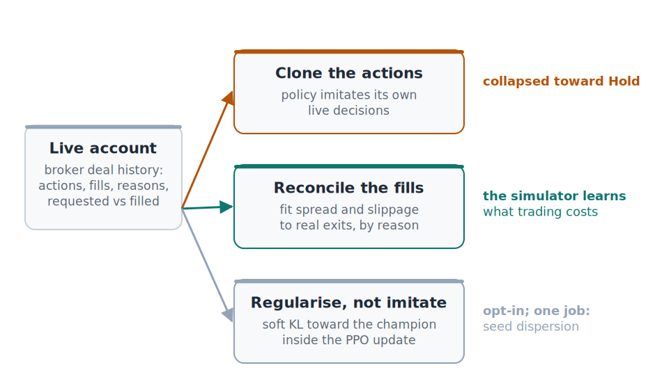
Figure 1. Only the first uses live data to change what the policy does; the other two change what the policy is trained in. This article is about why the first failed and how the other two replaced it.

What Behavioural Cloning Needs

Behavioural cloning is supervised learning on a policy: given observations and the actions a demonstrator took, fit the policy to reproduce those actions. It is the simplest form of imitation learning, and it has a well-known failure mode. When the cloned policy drifts into states the demonstrator never visited, it has no guidance and its errors compound. That problem is the subject of most of the imitation-learning literature, and it is not the problem I hit.

The problem I hit is prior to it. Cloning can only transfer knowledge the demonstrator has. Imitation helps when the demonstrator is better than the student (eg, a human expert, a stronger model, or a planner with extra information). If the demonstrator is the student itself, the demonstrations contain exactly what the student already knows, plus whatever noise the live environment added. If you weight demonstrations by trade outcomes and the policy has no edge, you end up selecting lucky trades and training the policy to repeat them.

I knew this argument when I built the loop. I built it anyway, for two reasons that seemed good at the time. First, the live account is the only place where execution is real: fills, slippage, stop orders triggered on real ticks. I thought some of that reality would transfer through the demonstrations. Second, the training environment starts each episode at a random point in history, and I hoped a few hundred steps of genuinely recent behaviour would anchor the policy to the current regime. Neither reason survives contact with the data, and I want to show the data rather than argue.

What I Built

The live trader logs every decision as an experience record: the observation, the action taken, and an info dictionary with the realised P&L, the lot size and the stop distance when a trade closes. The trainer reads those records at the start of every cycle, assembles them into episodes, and applies cloning in two places.

Step weights from trade outcomes

Each complete trade — open, holds, close — receives a weight from its R-multiple, the realised profit divided by the amount risked at the stop. Winners map to a weight between zero and one; losers get zero. The trade's weight is then spread evenly over every step of the trade, so a nine-bar trade contributes one open step, seven hold steps and one close step, all with the same weight. Steps outside any trade get zero. This is the part that matters most later. The listing is slightly condensed from the version that ran.

def compute_trade_cycle_step_weights(actions, infos, r_cap=3.0, eps=1e-8):
    """
    Non-negative BC weights based on trade R-multiple, debiased by trade length.
    For each complete trade (open ... close): R = realized_pnl / risk_at_SL,
    clamped to [-r_cap, r_cap]. Winners map to [0, 1]; losers get BC_LOSER_WEIGHT
    (default 0). The trade's weight is distributed equally across its steps.
    """
    n = len(actions)
    w = np.zeros(n, dtype=np.float32)
    in_trade, start = False, None
    loser_weight = float(CONFIG.get("BC_LOSER_WEIGHT", 0.0))

    for i, (a, info) in enumerate(zip(actions, infos)):
        info = info or {}
        if a in [1, 2] and not in_trade and info.get("trade_executed", False):
            in_trade, start = True, i
        if in_trade and a == 3 and info.get("trade_executed", False):
            end = i
            realized = float(info.get("realized_pnl") or 0.0)
            dyn_lot = float(info.get("dynamic_lot") or 0.0)
            sl_dist = float(info.get("sl_dist") or 0.0)
            risk = dyn_lot * CONTRACT_SIZE * sl_dist if (dyn_lot > 0 and sl_dist > 0) \
                   else 0.01 * CONFIG.get("INITIAL_BALANCE", 1.0)
            R = max(-r_cap, min(realized / (abs(risk) + eps), r_cap))
            trade_weight = R / r_cap if R >= 0 else loser_weight * (1.0 - abs(R) / r_cap)
            length = max(1, end - start + 1)
            w[start:end + 1] = trade_weight / length
            in_trade, start = False, None
    return w

A cloning step after every PPO rollout

A callback runs after every PPO rollout. It computes a weighted cross-entropy between the policy's action distribution and the demonstrated actions, applies an inverse-frequency class weight so that the rarer Buy, Sell and Close actions are not drowned out by Hold, and takes a gradient-clipped optimizer step. It also measures a KL proxy — the mean negative log-probability the policy assigns to the demonstrated actions — and when that exceeds 1.0, the cloning coefficient λ is decayed by ten percent, on the reasoning that a large disagreement means the demonstrations have drifted away from what the policy is doing. λ starts at 0.01. The listing is condensed from the version that ran.

class PPOBCLossCallback(BaseCallback):
    def __init__(self, live_episodes, lambda_bc=0.01, n_epochs=1, verbose=0,
                 kl_threshold=1.0, max_grad_norm=0.5):
        super().__init__(verbose)
        self.live_episodes = live_episodes
        self.lambda_bc = lambda_bc
        self.kl_threshold = kl_threshold
        self.max_grad_norm = max_grad_norm

    def _on_rollout_end(self):
        if not self.live_episodes:
            return True
        X = np.concatenate([ep["obs"] for ep in self.live_episodes])
        y = np.concatenate([ep["actions"] for ep in self.live_episodes])
        w = np.concatenate([compute_trade_cycle_step_weights(ep["actions"], ep["infos"])
                            for ep in self.live_episodes])

        # inverse-frequency class weights (alpha = 0.5) over positively weighted steps
        mask = w > 0
        counts = np.bincount(y[mask] if mask.any() else y, minlength=4).astype(np.float32)
        mean_count = counts[counts > 0].mean() if (counts > 0).any() else 1.0
        class_weights = (mean_count / (counts + 1e-6)) ** 0.5
        class_weights /= class_weights.mean() + 1e-8

        model = self.model
        model.policy.train()
        kl_values = []
        for start in range(0, len(X), 64):
            idx = np.random.permutation(len(X))[start:start + 64]
            obs = torch.tensor(X[idx], dtype=torch.float32, device=model.device)
            act = torch.tensor(y[idx], dtype=torch.long, device=model.device)
            sw = torch.tensor(w[idx], dtype=torch.float32, device=model.device)
            if sw.sum().item() < 1e-4:
                continue
            sw = sw * torch.tensor(class_weights, device=model.device)[act]
            sw = sw / sw.mean().clamp_min(1e-6).detach()

            logits = model.policy.get_distribution(obs).distribution.logits
            loss = (torch.nn.functional.cross_entropy(logits, act, reduction="none") * sw).mean()
            model.policy.optimizer.zero_grad()
            (self.lambda_bc * loss).backward()
            torch.nn.utils.clip_grad_norm_(model.policy.parameters(), self.max_grad_norm)
            model.policy.optimizer.step()

            with torch.no_grad():   # KL proxy: how far the demonstrations are from the policy
                logp = torch.log_softmax(logits, dim=-1)
                kl_values.append(float(-logp.gather(1, act[:, None]).mean()))

        mean_kl = float(np.mean(kl_values)) if kl_values else 0.0
        if mean_kl > self.kl_threshold:
            self.lambda_bc *= 0.9
        return True

A pre-training pass on the final model

The Optuna trials receive only the callback. The final model of each cycle — the one trained with the trial's best hyperparameters and evaluated on the validation window — receives something heavier first: two full epochs of weighted cloning over the entire live buffer, with the same class weights, through the policy's own optimizer, before PPO training begins. The intent was to warm-start the final model from the most recent live behaviour.

def behavioral_cloning(model, live_episodes, n_epochs=2):
    X = np.concatenate([ep["obs"] for ep in live_episodes])
    y = np.concatenate([ep["actions"] for ep in live_episodes])
    w = np.concatenate([compute_trade_cycle_step_weights(ep["actions"], ep.get("infos", []))
                        for ep in live_episodes])
    # ... same class weights as the callback ...
    model.policy.train()
    for epoch in range(n_epochs):
        for start in range(0, len(X), 64):
            idx = np.random.permutation(len(X))[start:start + 64]
            obs = torch.tensor(X[idx], dtype=torch.float32, device=device)
            act = torch.tensor(y[idx], dtype=torch.long, device=device)
            sw = torch.tensor(w[idx], dtype=torch.float32, device=device) * class_weights[act]
            sw = sw / sw.mean().clamp_min(1e-6).detach()
            logits = model.policy.get_distribution(obs).distribution.logits
            loss = (torch.nn.functional.cross_entropy(logits, act, reduction="none") * sw).mean()
            model.policy.optimizer.zero_grad()
            loss.backward()
            model.policy.optimizer.step()
    return model

That difference in dose — a light callback for trials, a heavy pass for final models — turned out to be the accidental comparison that makes the rest of this article possible.

How It Failed, First: The Buffer Died Quietly

The first failure has nothing to do with learning. It is an engineering failure, and I include it because it is the one most readers will actually hit.

Between the first article's model and the current one, I added a thirteenth feature. The observation grew from 212 to 228 numbers. The manifest contract described in the first article did its job: the live trader refused to load any model whose schema did not match. But the experience buffer had no such contract. Every episode the trader had logged before the change carried 212-dimensional observations, and the trainer, correctly, refused to clone from them. It logged a rejection and moved on — 3,412 times, over two months, on every cycle, for episodes it had rejected the cycle before. Nothing purged them.

The live buffer after the schema change

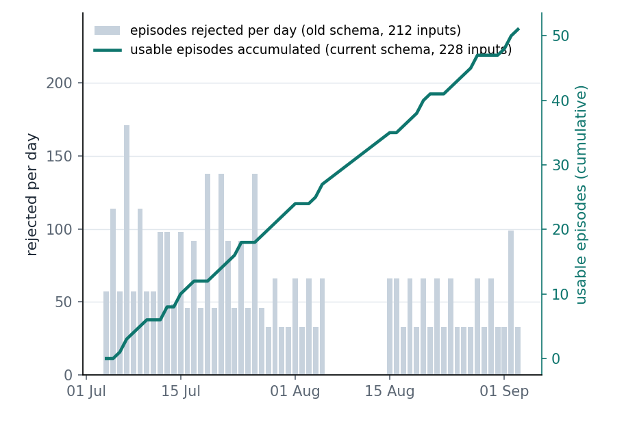
Figure 2. Bars: episodes rejected per day because they carried the old 212-input schema. Line: usable 228-input episodes accumulated as the live trader produced them. 3,412 rejections were logged in total; 51 usable episodes existed by the end.

As a result, the demonstration set was small: 51 live episodes, growing from 59 steps on 7 July to 3,554 by 3 September. That limits how far the results below can be generalised. A larger, older or differently composed buffer would contain different trades and a different mix of actions, and I have not tested what it would do. The small size is also the first item on the protocol at the end: an experience buffer needs the same schema contract as a model, and rejected records need to be deleted, not re-rejected forever.

How It Failed, Second: The Policy Learned to Do Nothing

Because usable episodes only began to exist on 7 July, the cloning loop was effectively switched on that day. That gives a before/after comparison: 16 final models trained and evaluated before cloning was active, and 67 after. It is not a randomised experiment. The 67 models after the switch all ran on one trainer version (188.3); the 16 before it span four minor versions (188.0 to 188.3), and the earliest four were trained on the previous 212-input observation. One further cycle, on 2 July, is excluded: its final evaluation crashed at shutdown, and the Sharpe the trainer logged for it was left over from the previous cycle, not measured. Models that never traded have no return variance; the trainer reports their Sharpe as 0.0, and they are counted as 0.0 below, not as negative.

One caveat applies to the metric itself. The trainer's final evaluation measures each final model on the validation window, and the final model is trained on the training and validation windows together, so the Sharpe ratios and Hold shares below are in-sample for the model being measured. Trials, by contrast, are evaluated on windows they were not trained on. This is the same on both sides of 7 July, so it does not bias the before/after comparison, but it is one more reason not to read the Sharpe levels as forecasts. I call it the evaluation window below, not a holdout.

Final-model outcome on the evaluation window	Before cloning (16 models)	Cloning applied (67 models)
Annualised Sharpe, median	+4.09	+1.21
Annualised Sharpe, median of models that traded	+4.09 (16)	+1.76 (55)
Annualised Sharpe, standard deviation	1.61	3.18
Models with negative Sharpe	0 of 16	18 of 67
Models that never traded	0	12
Passed every promotion gate	88%	42%
Hold share of decisions, median	44%	82%
Buy and Sell actions, median	5,782	431

Evaluation result of every final model

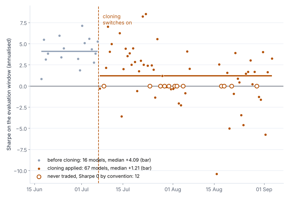
Figure 3. Evaluation-window Sharpe of every final model the trainer produced between 17 June and 3 September, one dot per model. The dashed line marks the first cycle with usable live episodes; horizontal bars are medians. Hollow markers are models that never traded, plotted at the trainer's conventional Sharpe of 0. The cycle of 2 July is not shown: its final evaluation failed, so its logged Sharpe was not a measurement.

The last two rows carry the clearest change. Before cloning, a final model held on a little under half its decisions. After cloning, the median model held on 82% of them, took about a thirteenth as many Buy and Sell actions, and twelve models never traded at all. Whatever else changed over the summer, the models that came out of the cloning loop traded far less.

Why the demonstrations may have taught inaction

Look again at the step-weight function. It gives a winning trade a weight and spreads that weight evenly across every step of the trade. The live trader's average holding time was 2.2 hours, about nine bars on M15. A nine-bar trade is one Buy or Sell, seven Holds and one Close, so seven-ninths of the weighted steps of such a trade say "Hold". The inverse-frequency class weight with exponent 0.5 halves that imbalance rather than removing it, and the final model then took two epochs of this through the policy's own optimiser, with no trust region to limit the step.

Here I have to be careful, because "Hold" means two different things. Inside a position it means keep the trade open; when flat it means do not open one. The observation tells the policy which state it is in. If every weighted trade looked like the nine-bar example, all of its Holds would be of the first kind, and the only weighted examples taken while flat would be the entries. Taken literally, such a dataset says "enter when flat, hold when in a trade", not "stop trading".

Reading the code again with that question in mind, the weighted set was not that clean. The step-weight function ends a trade only when it sees an executed Close from the agent. On the live account, a trade closed by the broker's stop-loss or take-profit, or by the maximum-holding rule, produces no such action: the trader simply finds the position gone at the next bar. The open segment then runs on through the flat bars that follow and through the next entry, until the agent itself closes a trade, and every step in it receives that last trade's weight. On a flat bar the trader logs either an entry or Hold, because a Close on a flat account is converted to Hold before it is logged, so those flat bars are almost all Holds. Over the account's history, 509 of its 934 exits were stop-loss or take-profit exits. So flat-state Holds did enter the weighted demonstrations, whenever a weighted segment spanned such an exit. I have not measured how many.

What the logs do show is that the change was in flat-state behaviour: fewer entries, and twelve models that never entered at all. My working explanation combines the two points above — a weighted dataset that is mostly Hold, part of it flat-state Hold by accident of the trade-boundary logic, fitted hard for two epochs without a trust region. It is consistent with the code and the logs, but this article does not prove it. Proving it needs the policy's Hold probability measured separately in flat and in-position states, before and after the pre-training pass.

It is worth being precise about what the R-multiple weighting did and did not do. It did not select for good entries in any way I can detect, because the demonstrator had no edge to select for. What it did was decide which stretches of live behaviour were cloned, and those stretches were not always the trades I thought they were.

The two doses

The strongest evidence that the change came from cloning, rather than from the market window or something else that drifted over the summer, comes from the two doses. Every Optuna trial and walk-forward evaluation in the same period received only the light callback — λ at most 0.01, gradient-clipped, one step per rollout. Only final models also received the heavy two-epoch pre-training pass. Across 4,107 trial and walk-forward evaluation episodes, the median Hold share moved from 21% before 7 July to 22% after. Across final models it moved from 44% to 82%, and 29 of the 67 final models after cloning held on more than nine decisions in ten.

This is not a comparison in which only the dose differs. Trials and final models differ in more than that: final models are trained once on the training and validation windows together, with the selected hyperparameters, and evaluated on the validation window, which is part of their own training data, while trials are evaluated out of sample. What makes the comparison useful is that those differences existed both before and after 7 July. The one change on that date that touched final models and not trials was the pre-training pass, and only final models moved. Restricted to the single trainer version that ran on both sides of the date (188.3), the picture is the same: trial episodes went from 18% to 22% Hold and final models from 52% to 82%, although only three final models fall on the before side of that comparison. What this design cannot rule out is something else that changed on 7 July and affected only the final models. I know of no such change, but I cannot exclude one.

Hold share by dose, before and after cloning

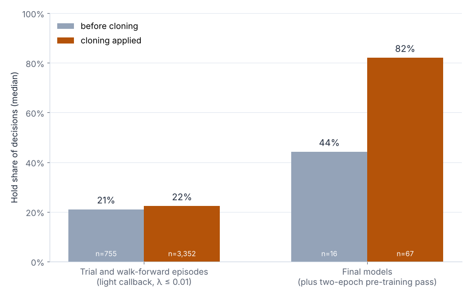
Figure 4. Median Hold share of decisions before and after cloning became active, with the number of episodes or models in each bar. Trial and walk-forward evaluations received only the light callback and barely moved. Final models also received the two-epoch pre-training pass and shifted toward Hold. The two groups differ in more than the dose, but those differences were present on both sides of 7 July.

One more number is worth reporting, with care. The callback logs a quantity the code calls a KL proxy. It is not a KL divergence: it is the mean negative log-probability the policy assigns to the demonstrated actions. Its average across the 67 cycles was 1.02, which corresponds to a geometric-mean probability of about 0.36 for the demonstrated action, against 0.25 for a uniform choice among four actions, so the policy agreed with the demonstrations more often than chance. The λ-decay guard fired 221 times and lowered the coefficient from 0.010 to an average of 0.007 by the end of a cycle, but its threshold of 1.0 sits almost exactly at that average, so the decays say more about where I set the threshold than about any conflict between cloning and PPO. I do not draw a conclusion from this number.

What this comparison cannot claim

The before group spans four trainer versions and a different stretch of the market; the walk-forward median Sharpe drifted from 3.40 to 2.97 across the boundary, so some of the decline in Sharpe belongs to the window. The absolute Sharpe levels also deserve little trust: as the next section shows, the simulator charged almost nothing for execution throughout this period, before and after cloning alike. Because both groups were trained and evaluated under the same cost model, that does not explain the difference between them, but it does mean neither +4.09 nor +1.21 estimates what these models would earn. One of the four promotions in the period happened during cloning, on 23 July, so cloning did not make promotion impossible. And the buffer was small and late-starting, so the operational failure above and the method itself are not fully separable here. What I am confident of is narrower: the shift toward Hold appears in final models only, only after 7 July, and not in the trials that ran alongside them. How much of the Sharpe decline is attributable to cloning alone, I do not know, and I have not tried to estimate it.

What Live Experience Actually Contains

Having removed cloning, I had to answer the question it was a bad answer to: what is a live account for, if not to teach the policy?

The answer came from a bug I found while reviewing the environment. The simulator's spread was set as SPREAD_PIPS * 0.0001 — a forex habit applied to gold, so a configured 0.30 became $0.00003 per side on a $4,600 instrument. Slippage was drawn symmetrically around zero, which makes it free on average, and its range was expressed in ATR units small enough to amount to about one cent. The policy in the first article had been trained in a world where trading cost nothing. Meanwhile the broker's records for the same account, read back through the reconciler described below, showed exit slippage of $2,467 across the 509 stop and target exits that carried it, about $4.85 per exit, close to a third of the realised profit.

That is what a live account contains that a simulator lacks: not information about where the market is going, but information about what it costs to act. Fills against requested prices. Which of stop and target actually triggered. Spread at the moment of exit, by session. None of that has anything to do with the policy's decisions, and all of it changes what the policy should learn.

The reconciler

So the live trader now does something simpler than logging demonstrations. Every few minutes it reads the broker's closed deals for its magic number, pairs each deal with the order that created it, and records requested versus filled. For an order the broker generated when a stop or target triggered, the order's price_open is the stop or target level itself, so those exits are measured exactly, with no hooks into the order-sending code. For market orders it depends on the broker. On my demo account the order history reports price_open as 0 for market orders, so none of the 934 entries and none of the 425 exits the agent closed itself carry a requested price. Of 1,868 reconciled deals, only the 509 stop-loss and take-profit exits have a measured slippage, and everything below is about those. Measuring entries on such a broker needs the trader to record the quote it saw when it sent the order; that is the next change.

def run(self):
    end = datetime.now() + timedelta(minutes=5)
    deals = mt5.history_deals_get(end - timedelta(days=self.lookback_days), end)
    for d in sorted(deals, key=lambda x: x.time):
        if d.magic != self.magic or int(d.ticket) in self._seen:
            continue
        if d.entry not in (mt5.DEAL_ENTRY_IN, mt5.DEAL_ENTRY_OUT):
            continue
        side = "in" if d.entry == mt5.DEAL_ENTRY_IN else "out"
        is_buy = d.type == mt5.DEAL_TYPE_BUY
        # direction of the POSITION: a buy deal opens a long; a sell deal closes a long
        direction = (1 if is_buy else -1) if side == "in" else (-1 if is_buy else 1)

        orders = mt5.history_orders_get(ticket=int(d.order))
        requested = float(orders[0].price_open) if orders else float("nan")
        filled = float(d.price)
        reason = self.REASON.get(getattr(d, "reason", -1), "other")   # sl / tp / expert / so

        # adverse slippage, positive = cost to us
        if side == "in":
            slip = (filled - requested) if direction == 1 else (requested - filled)
        else:
            slip = (requested - filled) if direction == 1 else (filled - requested)
        atr = self._atr_at(int(d.time))
        self._append_row(d, side, direction, reason, requested, filled, slip,
                         slip / atr, slip * d.volume * self.contract_size, atr)
        self._seen.add(int(d.ticket))

Four sign cases — opening long, opening short, closing long, closing short — and all four come out as a positive cost. The attachment includes a test against a fake broker for each case. The script also runs standalone, so you can point it at any account and see what your own exits cost before changing anything.

The calibration

At the start of every training cycle, the trainer reads the execution log and fits the simulator's cost ranges to it. The spread range becomes the 10th to 90th percentile of observed ask-minus-bid at decision time. The slippage range is fitted so that the simulator's mean adverse slippage matches the observed mean, in ATR units — exit slippage is heavy-tailed, and a fit on quartiles understates the cost that actually accrues. The fitted values go into a small JSON file that every training environment reads at construction — a detail that matters on Windows, where subprocess workers re-import the module and would never see a change to a variable in the parent. The manifest of every promoted model records the calibration it trained against.

def fit_execution_calibration(exec_path, spread_path, min_exits, min_spread, window_days):
    out = {"fitted_at": datetime.utcnow().isoformat(timespec="seconds")}
    cutoff = datetime.utcnow() - timedelta(days=window_days)

    ex = pd.read_csv(exec_path)
    ex = ex[(ex["side"] == "out") & (pd.to_datetime(ex["ts_utc"]) >= cutoff)]
    ex["adverse_atr"] = pd.to_numeric(ex["slip_atr"], errors="coerce").clip(lower=0.0)
    ex = ex.dropna(subset=["adverse_atr"])
    if len(ex) >= min_exits:
        # env: max ~ U(lo, hi) per episode, slippage ~ U(0, max) per trade -> expected cost (lo + hi) / 4.
        # Fit the MEAN (heavy tails make quartiles understate it) and let max vary +/-50% around it.
        mean_atr = float(ex["adverse_atr"].mean())
        out["SLIPPAGE_RANGE"] = (round(mean_atr, 5), round(max(3 * mean_atr, 1e-4), 5))
        out["n_exits"] = int(len(ex))
        out["exit_slip_atr_mean"] = round(mean_atr, 5)
        out["by_reason"] = ex.groupby("reason")["adverse_atr"].agg(["count", "mean"]).round(5).to_dict("index")

    sp = pd.read_csv(spread_path)
    sp = sp[pd.to_datetime(sp["ts_utc"]) >= cutoff]
    if len(sp) >= min_spread:
        p10, p90 = sp["spread"].quantile([0.10, 0.90])
        out["SPREAD_RANGE"] = (round(float(p10), 5), round(float(max(p90, p10 + 1e-4)), 5))
        out["n_spread"] = int(len(sp))
    return out

On the demo account, the first fit used 340 exits from the preceding 90 days: mean adverse slippage 0.055 ATR per exit, median 0.003. Across all 509 measurable exits since April the picture is the same — mean 0.053, median 0.003, thirty-seven percent filled at the stop or better, and the mean carried by the rest; the largest single exit slipped 3.25 ATR through its stop. The fitted range came out at (0.055, 0.165) ATR against the previous default of (0.0005, 0.002), whose implied mean of 0.0006 ATR was about eighty-five times below what the broker actually charged.

A first version of the fitter, on quartiles, gave (0.0, 0.030); with a distribution this skewed that still understated the mean by a factor of seven, which is why the fit targets the mean directly. The breakdown by reason across all 509 exits, shown in Figure 5, is the next refinement: stop-loss exits averaged 0.056 ATR adverse, take-profit exits 0.039 adverse but slightly favourable net, because targets are often filled through. The simulator currently applies one distribution to both; conditioning it on exit type is a small change now that the data says which way each leans.

Three limits are worth stating plainly. First, the calibration is fitted to stop-loss and take-profit exits only, for the reason above; entries and agent exits are not calibrated. Second, it matches the mean, not the shape. The simulator draws slippage from a bounded uniform range whose maximum is 0.165 ATR, while 5% of the measured exits slipped more than that and the worst 5% of exits carried 76% of all adverse slippage. Gap-like fills and stop-throughs are therefore still missing from training: the cost is right on average and wrong in the tail. Third, the fit targets adverse slippage only and the simulator charges it on every exit, while 72% of take-profit exits actually filled better than requested. Across the 509 measured exits the mean adverse slippage was 0.053 ATR and the net mean 0.029 ATR, so the simulator now charges about 1.8 times the net cost. I would rather the simulator err on the expensive side, but it is a bias, and it should be measured as one.

Even with those limits, this closes a loop that the cloning loop only pretended to close. The live account teaches the trainer something the trainer could not know, every cycle, and nothing about it depends on the demonstrator being good.

What exits actually cost, by reason

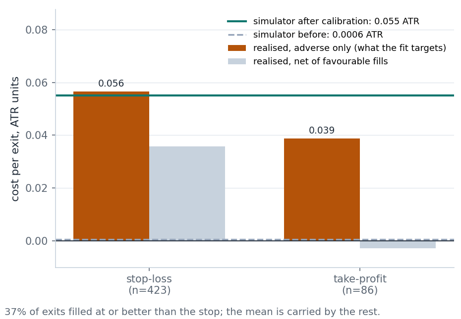
Figure 5. From the broker's own records for the demo account: 423 stop-loss and 86 take-profit exits. Dark bars are adverse slippage only, which is what the fit targets; light bars are net of favourable fills. The dashed line is the simulator's mean cost before calibration, the solid line after. Across all exits the adverse mean is 0.053 ATR against a median of 0.003 — 37% filled at or better than the stop, and the mean is carried by the rest. Costs are in ATR units so that volatility regimes are comparable.

Regularise, Don't Imitate

Cloning did one thing I still wanted: it tied each new model to the behaviour of the one before it. The first article showed why that matters — across 2,388 seed evaluations, validation Sharpe had a standard deviation of 3.16, and the same configuration could produce a Sharpe of +3.79 from one random seed and −4.47 from another. Something that pulls successive models toward a common behaviour has a legitimate job, as long as it does not also pull them toward doing nothing.

The replacement is a soft KL penalty toward the frozen champion. It runs alongside PPO rather than inside PPO's loss: after each rollout, it samples observations from the rollout buffer — the current training distribution, not a stale live buffer — computes the champion's action distribution on them, and takes one separate, small, gradient-clipped optimiser step on β times the KL divergence from the champion to the current policy. The differences from cloning are the ones that matter: soft targets rather than hard actions, so the policy is pulled toward the champion's probabilities rather than toward one demonstrated action (if the champion itself mostly holds, its targets will mostly say Hold too, so this softens class dominance without preventing it); the training distribution rather than live episodes, so there is no selection of trade segments; no outcome weighting, so it cannot chase lucky trades; and a guard that disables it if the champion's observation space differs.

class ChampionKLCallback(BaseCallback):
    def __init__(self, beta=0.02, manifest_path="models/manifest.json",
                 max_samples=4096, max_grad_norm=0.5, verbose=0):
        super().__init__(verbose)
        self.beta, self.manifest_path = float(beta), manifest_path
        self.max_samples, self.max_grad_norm = int(max_samples), max_grad_norm
        self.champion, self._tried = None, False

    def _load_champion(self):
        self._tried = True
        try:
            m = json.load(open(self.manifest_path, encoding="utf-8"))
            champ = PPO.load(m["model_path"], device=self.model.device)
            if tuple(champ.observation_space.shape) != tuple(self.model.observation_space.shape):
                return                       # KL between different input spaces is meaningless
            champ.policy.eval()
            for p in champ.policy.parameters():
                p.requires_grad_(False)
            self.champion = champ
        except Exception:
            pass                             # no champion: regulariser stays inert

    def _on_rollout_end(self):
        if self.beta <= 0:
            return True
        if self.champion is None and not self._tried:
            self._load_champion()
        if self.champion is None:
            return True
        obs = self.model.rollout_buffer.observations.reshape(-1, self.model.observation_space.shape[0])
        if len(obs) > self.max_samples:
            obs = obs[np.random.choice(len(obs), self.max_samples, replace=False)]
        x = torch.as_tensor(obs, dtype=torch.float32, device=self.model.device)
        with torch.no_grad():
            champ_logp = torch.log_softmax(self.champion.policy.get_distribution(x).distribution.logits, -1)
        self.model.policy.train()
        cur_logp = torch.log_softmax(self.model.policy.get_distribution(x).distribution.logits, -1)
        kl = (champ_logp.exp() * (champ_logp - cur_logp)).sum(-1).mean()
        self.model.policy.optimizer.zero_grad()
        (self.beta * kl).backward()
        torch.nn.utils.clip_grad_norm_(self.model.policy.parameters(), self.max_grad_norm)
        self.model.policy.optimizer.step()
        return True

I want to be careful about what I am claiming for this. It is switched off by default, because I have not yet measured it. It has one job — reduce seed-to-seed dispersion — and one test: run the walk-forward validation with β at zero and at 0.02 on the same folds and seeds, and compare the standard deviation of seed Sharpe. If it does not move that number, it comes out. I include the code because it is the shape the idea should take, not because it has earned its place yet. The first article's rule applies: nothing in this loop creates information that is not in the inputs. A regulariser can make the search less noisy; it cannot make the market more predictable.

Lessons and a Protocol

What I would tell someone about to build this loop

Cloning your own live trades is not a weak version of learning from experience. It is a different thing with the same name. In my system, with no directional edge in the demonstrator, it coincided with final models that stopped trading. Weighting by outcome did not help, because there was no edge for it to select; class reweighting softened the action imbalance without removing it. The pre-training pass, the part I thought was safe because it happened before PPO could react, is where the change appeared, and it was the part with no trust region.

The failure was visible from day one. On July 7, the first cloned final model had an evaluation-window Sharpe of −0.30 and an explained variance thousands below zero, which typically happens when the model produces near-zero return variance. I did not look, because the pipeline kept running and the gates kept rejecting, and rejections looked like the system working. They were. What I had not built was anything that asked why the rejection rate had doubled.

The protocol:

1. Give the experience buffer the same schema contract as the model. Store the observation dimension and feature hash with every episode. Refuse mismatches once, delete them, and count what remains. Fifty-one usable episodes is a number you want to know before you build anything on them.
2. Before cloning anything, look at the weighted demonstrations you are about to clone. Check where each weighted segment starts and ends, and take trade boundaries from the broker's position state, not from the agent's actions. Count actions separately for flat and in-position states. If the weighted set is dominated by Hold, expect the policy to drift toward Hold, and measure whether it does, in each state. These checks take a few lines.
3. Ask what the demonstrator knows that the student does not. If the demonstrator is the student, it adds no directional information. Imitation then cannot add edge, and, as here, it can add bias. Do not clone unless you can name what the demonstrator knows.
4. Use live data for what it uniquely contains: execution. Reconcile requested against filled prices from the broker's own records, by exit reason, and find out which deals your broker lets you measure. Fit the simulator's spread and slippage to that, check the tail as well as the mean, and record the calibration in the model's manifest.
5. If you want continuity between models, regularise toward the previous one alongside the RL update, with soft targets and a small coefficient, and give it one metric to move. If it does not move it, remove it.
6. When a gate's rejection rate changes, treat that as a signal, not as reassurance. The gates protected the account for two months while the thing feeding them was broken. They cannot tell you why.

Conclusion

The first article ended with a negative result about the market: gold's direction on M15 was not predictable from the features I had. This one ends with a negative result about one implementation of a method: in this pipeline, cloning the system's own live trades with outcome weighting and a heavy pre-training pass coincided with final models that stopped trading, and it did not add the edge it was meant to add. The failure was easy to miss because the safeguards kept working. The positive result is narrower and more useful. A live account is an instrument for measuring execution, and a simulator calibrated to real fills is a better place to train than one that is not, whatever the policy inside it ends up being able to learn.

This is not a claim that behavioural cloning is useless in trading, nor that self-imitation can never work. It is a claim about one form of self-imitation, measured over 83 final models, 51 usable live episodes and one account. Execution calibration is also not the only possible use of live data: off-policy diagnostics, regime labelling, risk calibration and action-conditional evaluation are all candidates I have not tested. If you have a demonstrator that is measurably better than your student on a forward window — a slower model, a human, a different information set — the calculus changes, and the protocol above tells you how to check. If you do not, execution is the one use I found for live data that clearly paid off.

References

1. Tuna, A. U. "Reinforcement Learning Meets MetaTrader 5: A Complete Pipeline for Training, Validating and Honestly Evaluating a Gold Trading Bot" MQL5 Articles, 2026. 
2. Pomerleau, D. "ALVINN: An Autonomous Land Vehicle in a Neural Network." NIPS (1989) — the original behavioural-cloning result
3. Ross, S., Gordon, G. and Bagnell, D. "A Reduction of Imitation Learning and Structured Prediction to No-Regret Online Learning." AISTATS (2011) — DAgger and compounding error
4. Schulman, J., et al. "Proximal Policy Optimization Algorithms." arXiv:1707.06347 (2017)
5. Stable Baselines3 Documentation
6. MQL5 Documentation

Files Attached to the Article

The archive unpacks into the terminal data folder, which opens from File → Open Data Folder in MetaTrader 5, and places four Python files, the three tables behind this article's results, and a pinned requirements list in MQL5\Files\RL_MT5_BC\. Every script runs as it is. test_reconciler.py needs no terminal at all and is the quickest way to see that the archive works; execution_reconciler.py measures what your own exits cost; calibration.py fits simulator ranges to that measurement; log_analysis.py prints this article's results table from the three CSV files, and builds the same files from your own trainer log. The two callbacks discussed in the article — the cloning loss and the KL regulariser that replaced it — are printed in the text above, condensed from the versions that ran. They are PPO callbacks that you drop into your own training loop rather than programs to run, so they are not in the archive.

#	File	Description
1	test_reconciler.py	Runs as-is, no terminal needed: checks the reconciler's four slippage sign cases against a fake broker. Start here.
2	execution_reconciler.py	Runs as-is against any MT5 account: pairs every deal with its order and records requested versus filled price, exit reason, ATR and adverse slippage in price, ATR and currency units, for every deal whose order carries a requested price.
3	calibration.py	Runs as-is on the reconciler's output: fits SPREAD_RANGE and SLIPPAGE_RANGE to real execution and writes the JSON the training environment reads.
4	log_analysis.py	Runs as-is. With --tables. it prints this article's results table from the three CSV files below; with --log it builds the same three files from your own trainer log. Final evaluations that failed are excluded.
5	final_models.csv	One row per final model in this article (84 cycles, the failed one flagged): the source of the results table and Figures 3 and 4.
6	trial_episodes.csv	One row per trial and walk-forward evaluation episode (4,107): the source of the trial bars in Figure 4.
7	buffer_timeline.csv	Schema rejections and usable live episodes per day: the source of Figure 2.
8	requirements.txt	Pinned library versions, identical to the first article's.
9	README.md	Maps each file to the section it comes from and gives the commands in order.
10	MQL5.zip	All of the above in a single archive. Unpack it into the terminal data folder and every file is placed in its required location: the archive already contains the MQL5\Files\RL_MT5_BC\ path. Then open a command prompt there, run pip install -r requirements.txt, and start with python test_reconciler.py.

Two sources are not included. The trainer log itself (52 MB) is left out; the three CSV files are everything extracted from it for this article. The demo account's broker deal records are left out because they are account records; execution_reconciler.py produces the same file for your own account.

Risk Disclaimer

Trading involves substantial risk of loss. Nothing in this article is investment advice. Past performance — simulated, demo or live — does not indicate future results.