Benchmark Champions vs. Real-World Optimization Problems

Table of Contents

1. Introduction
2. Requirements for Test Functions (Benchmarks)
3. Modifying Test Functions to Filter Out Duds
4. Conclusions

Introduction

You run dozens of population-based optimizers on the same test bench and see a neat table of top performers. The problem is that some of these victories do not reflect the algorithm’s true search power: a high result may stem not from the algorithm’s ability to find the optimum, but from a coincidence between the geometry of the algorithm’s steps and the geometry of a specific test function. A maximum located on the boundary, at the center, or near the diagonal of the normalized space gives certain classes of methods a systematic advantage.

In this article, we formalize this risk, especially the “diagonal effect,” provide a measurable diagnostic criterion, and show how to eliminate structural advantages from a benchmark set. After reading this, you will get not an abstract diagnosis, but concrete tools: a rule for checking the position of an extremum, a procedure for verifying RAW extrema (VerifyExtremes.mq5), and an example of practical correction of test functions.

Spiral Dynamics Optimization (SDO) Algorithm

The article on the SDO algorithm provided a detailed analysis of the following mechanism. The original SDO algorithm, proposed by Tamura and Yasuda in 2011, uses pairwise coupling of coordinates when moving agents in multidimensional space: a separate two-dimensional rotation spiral is constructed for each pair of coordinates. The test functions in our series, in their multidimensional form, are structured as multiple copies of two-dimensional functions — with exactly the same pairwise structure. The conclusion was already explicitly stated in the article’s analysis of the algorithm: “Since the articles use multidimensional functions made up of repeated two-dimensional functions, the original SDO may show unjustifiably high results, because it uses pairwise coupling of coordinates. Thus, in other multidimensional problems where the coordinates are not related to one another in any way, the spiral algorithm will yield poor results. In other words, for the spiral algorithm in this example, artificially favorable conditions will inadvertently be created on the duplicated functions.

The decision made then was to replace the pairwise spiral rotation with the projection of a two-dimensional spiral onto a single coordinate axis. In the modified version of SDOm, each coordinate was updated independently according to the damped harmonic oscillation formula: x(t) = A·e^(−γt)·cos(ωt + φ), which completely eliminated coupling between coordinates and removed the artificially favorable conditions. The algorithm became fair, but the result, of course, declined — SDOm ranked 8th out of 23 algorithms.

This case demonstrated an important principle: when the internal geometry of the algorithm (the pairwise coupling of coordinates) coincides with the geometry of the test function (a pairwise duplicated two-dimensional structure), the algorithm scores points not through optimization, but because of this coincidence.

Modified Dingo Optimization Algorithm (DOAm)

In the article on the DOA modification, DOAm demonstrated a characteristic asymmetry in its results: an outstanding score on the Forest function — and a significantly weaker result on the Hilly function. Such a discrepancy between the results on two functions of the same test bench is a reliable indicator: the algorithm may not possess universal optimization power, but may instead structurally match one specific test function. The matching mechanism in the case of DOAm may differ from that of SDO, but the pattern is the same — and it is precisely this pattern that drew our attention to the need for a more in-depth analysis.

After reading this, you will know exactly how to tell a true “detective” from a polished dud among optimization algorithms.

Requirements for Test Functions (Benchmarks)

The question of the properties of test functions was raised as early as the test bench design phase. In the article on the Grey Wolf Optimizer (GWO), four key conditions were identified that test functions must satisfy in order to eliminate unintended advantages for the algorithms under test.

First condition: the global extremum must not be located on the boundary of the domain. The search strategies of many algorithms do not include mechanisms for handling cases where optimized parameter values go outside the permissible range; hard clipping at the edges of permissible ranges is always added to the code artificially in order to enforce the search boundaries. If the global maximum is located on the boundary, such an algorithm may accidentally “run into” it when it overshoots the allowable range — and produce an excellent result that has nothing to do with the quality of the search. A high score is not the result of optimization, but rather a side effect of the lack of boundary checks.

Second condition: the global extremum must not be located at the center of the coordinate range. This point deserves a detailed analysis, since violating it leads to one of the most common — and yet most subtle — forms of “cheating.”

Third condition: the global minimum must be close to the center of the range. This is the mirror counterpart to the second condition: averaging the coordinates must not produce an advantage under any circumstances.

Fourth condition: the mean value of the surface must be significantly below the 50% level of the [min; max] range. Otherwise (especially when there are many variables), random coordinates may yield a result of about 50% of the maximum or higher.

Three of the four conditions were fully satisfied when designing the series of test functions: Hilly, Forest, and Megacity (the third condition is practically satisfied; the center of the search range is very close to the point of the global minimum). However, as algorithm testing has shown, this list turned out to be incomplete. There is another structural feature that allows certain algorithms to systematically achieve unjustifiably high scores.

Why should an extremum not be at the center of the range?

This question seems obvious, but the mechanism behind it is worth examining in detail, because it is by analogy with it that we will discover a new type of “cheating.”

There is an entire class of algorithms in which the coordinates of agents tend toward the midpoint of the range. The reasons vary: (1) uniform initialization followed by convergence toward the center of mass; (2) averaging the positions of several agents; (3) symmetric increments with zero expected value, which, with a sufficient number of iterations, lead to a drift toward the center of the range.

If the global maximum of the test function is located at the geometric center of the domain, all of these algorithms gain a systematic advantage: their agents either begin optimization already near the goal or inevitably drift toward it without performing any meaningful search. In this case, the ranking table measures not search ability, but the extent to which the algorithm tends toward the center.

The decision was made back when the test bench was being designed: the global maximum is shifted away from the center of the range, while the global minimum, conversely, is placed closer to the center — to ensure that averaging the coordinates leads to the worst result rather than the best one. This principle remains fundamental.

But what is the analogy with the problem we discovered later? It is that the “center of the range” is only one of several privileged geometric structures. The diagonal of the space is another. And just as an extremum at the center helps algorithms that average coordinates, an extremum on the diagonal helps algorithms with homogeneous coordinate updates.

What is the diagonal effect, and why is it dangerous?

The HHO (Harris Hawks Optimization) algorithm, proposed in 2019 and implemented in our previous article, was the catalyst that led to the formulation of a new requirement for test functions. The “cheating” mechanism here is not related to either pairwise coupling of coordinates (as in SDO) or any specific search strategy — it is more fundamental and affects an entire class of algorithms.

A key element of HHO is the scalar “escape energy” E, which decreases from ±2 to zero as the iteration budget is consumed: E = 2·E₀·(1 − t/T), where E₀ ~ U(−1, 1) is a random initial energy. When |E| ≥ 1, the algorithm operates in exploration mode; when |E| < 1, it switches to the attack phase, which includes four strategies. This is where the root of the problem lies: in most attack strategies, the factor E is applied to all coordinates simultaneously as a single scalar coefficient.

Let us examine this using specific formulas from the implementation. Strategy 2 (hard besiege, r ≥ 0.5, |E| < 0.5) is expressed as:

X_next[i] = X_prey − E · |X_prey − X[i]|

Here, E is the same number for all coordinates. This means that if the agent is at the point (0.3, 0.5) and the “rabbit” (the best solution) is at the point (0.6, 0.8), then the increment in each coordinate is proportional to the same value, E. Geometrically, the agent moves in a straight line from its current position to the target. Strategy 1 (soft besiege) uses the formula X_next[i] = (X_prey − X[i]) − E·|J·X_prey − X[i]|, where J is the “rabbit’s” jump strength, but E remains the same for all coordinates. Strategies 3 and 4 add Lévy flight, but only as a fallback maneuver — the main candidate Y is calculated using the same formulas with the same scalar E.

There is also a second factor that exacerbates the problem: classical HHO lacks an agent personal best component (pbest). All agents are guided by a single global best solution — the “rabbit” (X_prey). This means that the entire swarm moves toward the same point, generating a bundle of correlated diagonal trajectories. In the article on HHO, we explicitly pointed this out: “the narrow ‘needle’ of the global maximum requires the accumulation of the agent’s personal experience (the personal best component), which classical HHO lacks — and the algorithm’s diagonally correlated steps generally do not hit it.”

Visualization in the 3D test bench clearly confirmed this: throughout the optimization process, the agents’ movements remain linear and oriented at the same angle. This motion in itself is not a defect, but rather a normal search mechanism: the agent moves toward the goal along the shortest path. The problem arises when the structure of the test function matches this mechanism.

In its original form, the Forest function has a maximum in normalized coordinates at x_norm ≈ 0.591 and y_norm ≈ 0.731. The distance from this point to the main diagonal y = x is only |0.731 − 0.591| = 0.140. The maximum lies almost on the diagonal. Correlated diagonal HHO trajectories are highly likely to cross the region of attraction of this maximum: a cluster of agents converging on the “rabbit” inevitably combs through the vicinity of the global optimum. The result is consistently high performance, virtually independent of the problem dimensionality: 0.929 for 5 × 2 = 10 variables, 0.960 for 25 × 2 = 50, and 0.951 for 500 × 2 = 1,000 — absolute first place among 45 algorithms on this function.

The picture for the Hilly function is the exact opposite. The Hilly maximum is a narrow Gaussian peak with a width of approximately 0.3 units, located at the normalized coordinates x_norm ≈ 0.253 and y_norm ≈ 0.604. The difference |0.604 − 0.253| = 0.351 — the maximum is well away from the diagonal. The diagonal trajectories of the HHO agents pass by this peak. The absence of a personal best (pbest) prevents the algorithm from “remembering” random close approaches to the needle and returning to them. As a result, HHO yields 0.585, 0.406, and 0.342 for 10, 50, and 1,000 variables, respectively — values that are nearly indistinguishable from random search (random walk yielded 0.488, 0.322, and 0.258 on the same function). HHO ranks last among all algorithms in the table for this function — and at the same time ranks absolute first on Forest.

It is precisely this contrasting combination that serves as a diagnostic indicator of “cheating.” In our article on the HHO implementation, we had already recorded the following conclusion: “the top ranking is not due to universal effectiveness, but rather to the partial ‘compatibility’ of the algorithm’s mechanics with the structure of a specific benchmark.” The final score of 68.32% and the formal first place in the table resulted not from optimization capabilities, but from structural resonance with a single function: Forest gave HHO 2.841 out of a possible 3.0 points, while Hilly gave it only 1.333 out of 3.0. Without the anomalous result on Forest, the algorithm would have ranked in the bottom half of the table.

An analysis of three cases — SDO with pairwise coupling of coordinates, DOAm with asymmetry in the Forest/Hilly results, and HHO with the diagonal effect — leads to a general conclusion. The two existing requirements (the extremum is neither on the boundary nor at the center) must be supplemented by one more:

The global extremum must be located away from the main diagonals of the normalized search space

Specifically: the normalized coordinates x_norm and y_norm of the global maximum should not be close to each other. Practical threshold: |x_norm − y_norm| > 0.3.

Why the diagonal specifically? In many algorithms, all coordinates are updated in proportion to the same scalar quantity: (target − current position), multiplied by a common coefficient. This holds true not only for HHO with its “escape energy” E: any algorithm in which the step along each coordinate is determined by a single scalar multiplier (a common contraction coefficient, a uniform convergence rate, or a common inertia parameter) de facto moves agents along diagonal directions. If the maximum of the test function lies near the diagonal, all such algorithms gain an undeserved advantage — just as algorithms with uncontrolled boundaries gain an advantage when the maximum is located at the edge of the range, and just as algorithms that average coordinates gain an advantage when the maximum is located at the center.

These three requirements now form a closed system of safeguards against the three main classes of structural coincidences:

The extremum is not on the boundary — this rules out the advantage of algorithms with defective boundary control, whose coordinates “spill over” the edge of the range and accidentally land at the maximum.

The extremum is not at the center — this rules out the advantage of algorithms whose agents tend to average their coordinates across the range, whether through symmetric initialization, averaging the positions of multiple agents, or symmetric random increments with a zero expected value.

The extremum is not on the diagonal — this rules out the advantage of algorithms with uniform coordinate scaling, which move agents toward the target proportionally across all dimensions at once, producing straight diagonal trajectories in normalized space.

Each of these requirements closes a specific “cheating” channel — a situation in which the algorithm’s mechanics resonate with the structure of the test function, creating the illusion of high-quality optimization. All modifications to the Forest and Megacity functions described below are governed by this third condition.

Modification of Test Functions

The purpose of this modification is not to change the nature of the functions, but to eliminate the geometric advantage that algorithms using diagonal trajectories gain for free. The functions should remain just as difficult to search, but should no longer be “convenient” for a specific mechanism. The Hilly function was not changed — its maximum is already sufficiently far from the diagonal (|x_norm − y_norm| = 0.351). Two different approaches were used for the remaining two functions: for Forest, shifting the boundaries of the domain (the search window) while keeping the formula unchanged; for Megacity, changing the formula while preserving the overall structure.

Forest

The original function is built on a basic oscillating background a + b raised to the fourth power, with two Gaussian peaks added — a broad one (σ = 0.9) and a narrow one (σ = 0.3) — as well as a negative Gaussian term that forms a minimum. The Core() formula has not changed in the modified version — all coefficients, centers, and Gaussian sigmas remain the same. The boundaries of the domain have changed — the search window has been shifted:

Parameter	Original	Modification
xMinRange	−43.50	−42.50
xMaxRange	−39.00	−37.00
yMinRange	−47.35	−45.00
yMaxRange	−40.00	−39.80

Expanding the window to the right (xMaxRange from −39 to −37) brought a different maximum of the base oscillation (a+b)⁴ into the viewing area, with a significantly higher raw value: raw_max = 3.027 instead of the previous 1.878. The global maximum shifted from the point (−40.84, −41.98) to the point (−37.70, −41.98). The normalized coordinates changed: in the original, x_norm ≈ 0.591, y_norm ≈ 0.731, Δ = 0.140 — the maximum is almost on the diagonal.

In the modified version, x_norm ≈ 0.873, y_norm ≈ 0.580, and Δ = 0.293 — the maximum is far from the diagonal, although it does not reach the formal threshold of 0.3. Nevertheless, as the test results will show, even this shift is enough to cause a sharp drop in HHO results — which confirms the sensitivity of diagonal algorithms to the position of the maximum.

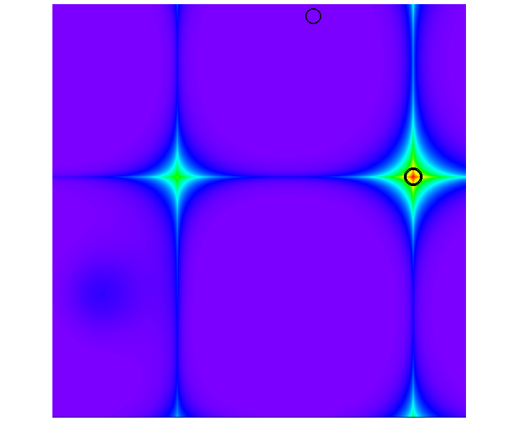
Forest Test Function

In this form, the Forest function is now included in the library of test functions.

//——————————————————————————————————————————————————————————————————————————————
class C_Forest : public C_Function
{
public: //===================================================================
  C_Forest ()
  {
    fuName = "Forest";

    //function boundaries
    xMinRange = -42.50;
    xMaxRange = -37;
    yMinRange = -45;
    yMaxRange = -39.8;

    //maximum coordinates
    globalMaxFunValue = 1.0;  // raw: 3.0269632693877031
    xGlobalMax        = -37.6991104999996764;
    yGlobalMax        = -41.9822944000032692;

    //minimum coordinates
    globalMinFunValue = 0.0;  // raw: 0.0000000000000000
    xGlobalMin        = -39.0288234999996675;
    yGlobalMin        = -39.9586780000031325;
  }

  double Core (double x, double y)
  {
    double a = MathSin (MathSqrt (MathAbs (x - 1.13) + MathAbs (y - 2.0)));
    double b = MathCos (MathSqrt (MathAbs (MathSin (x))) + MathSqrt (MathAbs (MathSin (y - 2.0))));
    double f = a + b
               + 1.01 * exp (-(pow (x + 42, 2) + pow (y + 43.5, 2)) / 0.9)
               + 1.0  * exp (-(pow (x + 40.2, 2) + pow (y + 46, 2)) / 0.3);

    double res = MathPow (f, 4)
                 - 0.3  * exp (-(pow (x + 42.3, 2) + pow (y + 46.0, 2)) / 0.02);

    //return res;
    return Scale (res, 0.0000000000000000, 3.0269632693877031, 0.0, 1.0);
  }
};
//——————————————————————————————————————————————————————————————————————————————

Megacity

The original function is built on the same base pair a + b as Forest, but after raising it to the fourth power, floor() is applied, creating a discrete, stepped landscape. The global maximum is determined by the points where sin(x) = 0 and sin(y−2) = 0 simultaneously, that is, x = nπ and y = 2 + mπ. The point closest to the center had normalized coordinates x_norm ≈ 0.858, y_norm ≈ 0.610, and a distance from the diagonal of 0.248 — not far enough.

In the modified version, the center of function a is shifted: (x + 10.13) is used instead of (x − 1.13), and (y − 5.0) is used instead of (y − 2.0). This shifts the regions where a reaches its maximum to another part of the search space. Normalized coordinates of the new maximum: x_norm ≈ 0.072, y_norm ≈ 0.610, distance from the diagonal: 0.538. The maximum has shifted to the left side of the space — diagonal trajectories oriented along the y ≈ x axis hardly ever reach that region. The value of raw_max changed from 12 to 14 — because at the new point, the base function has a different value, and floor((a+b)⁴) yields a different result. That is precisely why RAW scanning was necessary during verification: without it, Scale() would have been calibrated to the wrong range.

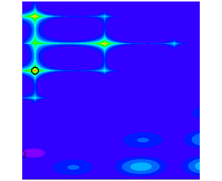
Megacity Test Function

The Megacity function is now included in the test function library in this form.

//——————————————————————————————————————————————————————————————————————————————
class C_Megacity : public C_Function
{
public: //===================================================================
  C_Megacity ()
  {
    fuName = "Megacity";

    //function boundaries
    xMinRange = -10.0;
    xMaxRange = -2;
    yMinRange = -10.5;
    yMaxRange = 10;

    //maximum coordinates
    globalMaxFunValue = 1.0;
    xGlobalMax        = -9.428;
    yGlobalMax        = 2.0009;

    //minimum coordinates
    globalMinFunValue = 0.0; //-1
    xGlobalMin        = -10.0;
    yGlobalMin        = -7.66485;
  }

  double Core (double x, double y)
  {
    double a = MathSin (MathSqrt (MathAbs (x + 10.13) + MathAbs (y - 5.0)));
    double b = MathCos (MathSqrt (MathAbs (MathSin (x))) + MathSqrt (MathAbs (MathSin (y - 2.0))));
    double f = a + b;

    double res = floor (MathPow (f, 4)) -
                 floor (2 * exp (-(pow (x + 9.5, 2) + pow (y + 7.5, 2)) / 0.4));

    if (res < -1.0) res = -1.0;

    return Scale (res, -1.0, 14.0, 0.0, 1.0);
  }
};
//——————————————————————————————————————————————————————————————————————————————

Final comparison of the normalized coordinates of the maxima:

Function	x_norm (original)	y_norm (original)	Δ orig.	x_norm mod.	y_norm mod.	Δ mod.
Hilly	0.253	0.604	0.351	unchanged
Forest	0.591	0.731	0.140	0.873	0.580	0.293
Megacity	0.858	0.610	0.248	0.072	0.610	0.538

Hilly already met the criterion Δ > 0.3 and remained unchanged. Megacity exceeds the threshold by a wide margin (Δ = 0.538). Forest does not formally reach the 0.3 threshold; however, Δ doubled — from 0.140 to 0.293 — and, as the test results will show, this proved sufficient to cause the HHO results to collapse. This observation suggests that the 0.3 threshold is not an absolute limit, but rather a guideline: the sensitivity of a particular algorithm to the position of the maximum relative to the diagonal depends on its mechanics.

Verification of Modified Functions

The VerifyExtremes.mq5 helper script was developed to accurately determine the extrema of modified functions and visually verify them. It performs three tasks at once: determines the exact raw values raw_min and raw_max for the function before Scale(), draws a heat map of the function directly on the MetaTrader 5 chart (identical to the visualization in the main test bench), and verifies the correctness of the calibration via CalcFunc().

The need for this script stems from the class architecture in TestFunctions.mqh: the Core() method always returns a result that has already been normalized via Scale(). To find the actual raw_min and raw_max values for calibration, you need to compute res before Scale() — this is exactly what the CoreRaw_*() functions do; their bodies exactly replicate Core(), except for the last line.

The verification procedure following any modification to a function consists of two runs. The first run scans the RAW values across a GridN×GridN grid (a value of 10,000 yields 100 million points — enough to accurately locate any extremum) and outputs ready-to-use code snippets to the log for insertion into the class constructor and Core(). For example, for Megacity, the result looks like this:

--- insert into the class constructor ---
globalMaxFunValue = 1.0; // raw: 14.0000000000000000
xGlobalMax = -9.4280000000000008;
yGlobalMax = 2.0009000000000015;
globalMinFunValue = 0.0; // raw: -1.0000000000000000
xGlobalMin = -10.0000000000000000;
yGlobalMin = -7.6648499999999995;

--- insert into Core() ---
return Scale (res, -1.0000000000000000, 14.0000000000000000, 0.0, 1.0);

These lines are copied into TestFunctions.mqh, and the file is recompiled. The second run verifies the calibration: the script calls CalcFunc() with the updated coordinates and checks that the function returns 1.0 at the maximum point and 0.0 at the minimum point.

CalcFunc CHECK (applicable after inserting the new Scale() calls):
CalcFunc at the max point = 1.00000000 (should be approximately 1.0)
CalcFunc at the min point = 0.00000000 (should be approximately 0.0)

If both values match, calibration is complete and you can begin testing the algorithms. If the script displays the warning “⚠ max is far from 1.0,” this means either that TestFunctions.mqh has not been recompiled, or that the found point lies on the boundary of a discrete floor() cell and is unstable — in this case, simply shift xGlobalMax by a few thousandths toward the center of the cell.

The heat map is generated in parallel with the calculations using CCanvas. The HSL color scheme is identical to that of the main test bench: blue represents minimum values, green represents average values, and red represents maximum values. The maximum is marked with a large black circle, and the minimum with a small one. A heat map immediately shows whether a peak is sharp, whether it is located where it should be, and whether there are any competing peaks of comparable height. If the global maximum is far from the main diagonals, the conditions for a fair comparison of algorithms are met.

//——————————————————————————————————————————————————————————————————————————————
// RAW functions — res before Scale().
// *** SYNCHRONIZE the bodies with Core() in TestFunctions.mqh ***
//——————————————————————————————————————————————————————————————————————————————
double CoreRaw_Forest (double x, double y)
{
  double a = MathSin (MathSqrt (MathAbs (x - 1.13) + MathAbs (y - 2.0)));
  double b = MathCos (MathSqrt (MathAbs (MathSin (x))) + MathSqrt (MathAbs (MathSin (y - 2.0))));
  double f = a + b
             + 1.01 * MathExp (-(MathPow (x + 41.5, 2) + MathPow (y + 46.0, 2)) / 0.9)
             + 3.0  * MathExp (-(MathPow (x + 41.5, 2) + MathPow (y + 46.0, 2)) / 0.3);
  return MathPow (f, 4)
         - 0.3 * MathExp (-(MathPow (x + 42.3, 2) + MathPow (y + 46.0, 2)) / 0.02);
}

//+------------------------------------------------------------------+
//|                                                                  |
//+------------------------------------------------------------------+
double CoreRaw_Megacity (double x, double y)
{
// *** SYNCHRONIZED with Core() in TestFunctions.mqh ***
  double a   = MathSin (MathSqrt (MathAbs (x + 10.13) + MathAbs (y - 5.0)));
  double b   = MathCos (MathSqrt (MathAbs (MathSin (x))) + MathSqrt (MathAbs (MathSin (y - 2.0))));
  double f   = a + b;
  double res = MathFloor (MathPow (f, 4))
               - MathFloor (2.0 * MathExp (-(MathPow (x + 9.5, 2) + MathPow (y + 7.5, 2)) / 0.4));
  if (res < -1.0) res = -1.0;
  return res;
}

//+------------------------------------------------------------------+
//|                                                                  |
//+------------------------------------------------------------------+
double CoreRaw_Hilly (double x, double y)
{
  return 20.0 + x*x + y*y
         - 10.0 * MathCos (2.0*M_PI*x) - 10.0 * MathCos (2.0*M_PI*y)
         - 30.0  * MathExp (-(MathPow (x-1.0,       2) + y*y) / 0.1)
         + 200.0 * MathExp (-(MathPow (x+M_PI*0.47, 2) + MathPow (y-M_PI*0.2, 2)) / 0.1)
         + 100.0 * MathExp (-(MathPow (x-0.5,       2) + MathPow (y+0.5,      2)) / 0.01)
         - 60.0  * MathExp (-(MathPow (x-1.33,      2) + MathPow (y-2.0,      2)) / 0.02)
         - 40.0  * MathExp (-(MathPow (x+1.3,       2) + MathPow (y+0.2,      2)) / 0.5)
         + 60.0  * MathExp (-(MathPow (x-1.5,       2) + MathPow (y+1.5,      2)) / 0.1);
}

//+------------------------------------------------------------------+
//|                                                                  |
//+------------------------------------------------------------------+
double CoreRaw (EFunc f, double x, double y)
{
  switch (f)
  {
  case Forest:
    return CoreRaw_Forest   (x, y);
  case Megacity:
    return CoreRaw_Megacity (x, y);
  case Hilly:
    return CoreRaw_Hilly    (x, y);
  default:
    return 0.0;
  }
}
//——————————————————————————————————————————————————————————————————————————————

The block above is needed for one reason: the function classes in TestFunctions.mqh do not provide access to the raw value of `res` — the `Core()` method always returns the result already normalized via `Scale()`. To find the actual raw_min and raw_max values for calibration, you need to calculate res before Scale() — and that is exactly what the CoreRaw_*() functions do.

Why only three and not all of them? Because the script was created specifically to verify modified functions. In our study, only Forest and Megacity were modified. Hilly has been added for completeness as a reference point — it has not changed, and its RAW values are already known.

For the other functions in EFunc — Rastrigin, Ackley, Rosenbrock, Peaks, and others — RAW scanning is not necessary in the context of this study. If you need to modify any of them in the future, simply add the corresponding CoreRaw_*() function and a line to the switch statement. The pattern is always the same: copy the body of Core() from the class, remove the last line `return Scale(...)`, and return `res` directly.

//——————————————————————————————————————————————————————————————————————————————
// The HSL palette is identical to that of the series’ main test bench
// (DoubleToColor: loH=0, upH=270, Revers=true)
//——————————————————————————————————————————————————————————————————————————————
double HueToRGB (double v1, double v2, double vH)
{
  if (vH < 0) vH += 1;
  if (vH > 1) vH -= 1;
  if ((6*vH) < 1) return v1 + (v2-v1)*6*vH;
  if ((2*vH) < 1) return v2;
  if ((3*vH) < 2) return v1 + (v2-v1)*(2.0/3-vH)*6;
  return v1;
}

//+------------------------------------------------------------------+
//|                                                                  |
//+------------------------------------------------------------------+
color HSLtoRGB (int h, double s, double l)
{
  if (s == 0.0)
  {
    int c = (int)(l*255);
    return StringToColor ((string)c+","+(string)c+","+(string)c);
  }
  double v2  = (l < 0.5) ? (l*(1.0+s)) : ((l+s)-(l*s));
  double v1  = 2.0*l - v2;
  double hue = (double)h / 360.0;
  int r = (int)(255 * HueToRGB (v1, v2, hue + 1.0/3.0));
  int g = (int)(255 * HueToRGB (v1, v2, hue));
  int b = (int)(255 * HueToRGB (v1, v2, hue - 1.0/3.0));
  return StringToColor ((string)r+","+(string)g+","+(string)b);
}

// t ∈ [0,1] → color; Revers=true as in the test bench: max→red (h=0), min→blue (h=270)
uint FuncColor (double t)
{
  t = MathMax (0.0, MathMin (1.0, t));
  int h = (int)((1.0 - t) * 270.0);
  return COLOR2RGB (HSLtoRGB (h, 1.0, 0.5));
}
//——————————————————————————————————————————————————————————————————————————————

//——————————————————————————————————————————————————————————————————————————————
// Heat map — calls Core() (with Scale), renders [0,1] using HSL
//——————————————————————————————————————————————————————————————————————————————
void DrawHeatmap (C_Function &fn, CCanvas &cv, int sz)
{
  double xMin  = fn.GetMinRangeX (), xMax = fn.GetMaxRangeX ();
  double yMin  = fn.GetMinRangeY (), yMax = fn.GetMaxRangeY ();
  double stepX = (xMax - xMin) / (sz - 1);
  double stepY = (yMax - yMin) / (sz - 1);

  for (int px = 0; px < sz; px++)
  {
    double x = xMin + px * stepX;
    for (int py = 0; py < sz; py++)
    {
      double y = yMax - py * stepY;          // py=0 → yMax (top), as in the test bench
      double v = fn.Core (x, y);             // Core() is already normalized to [0,1]
      cv.PixelSet (px, py, FuncColor (v));
    }
    if (px % 60 == 0)
      Comment (fn.GetFuncName (), " rendering  ", DoubleToString (100.0*px/sz, 0), "%");
  }

// maximum marker — black ring (as in the test bench)
  int mxPx = (int)MathRound ((fn.GetMaxFuncX () - xMin) / stepX);
  int mxPy = (int)MathRound ((yMax - fn.GetMaxFuncY ()) / stepY);
  for (int r = 10; r <= 13; r++)
    cv.Circle (mxPx, mxPy, r, COLOR2RGB (clrBlack));

// minimum marker — smaller black ring
  int mnPx = (int)MathRound ((fn.GetMinFuncX () - xMin) / stepX);
  int mnPy = (int)MathRound ((yMax - fn.GetMinFuncY ()) / stepY);
  for (int r = 10; r <= 11; r++)
    cv.Circle (mnPx, mnPy, r, COLOR2RGB (clrBlack));

  Comment ("");
}
//——————————————————————————————————————————————————————————————————————————————

//——————————————————————————————————————————————————————————————————————————————
// RAW scanning (before Scale())
//——————————————————————————————————————————————————————————————————————————————
void ScanRaw (EFunc funcType, C_Function &fn, int N,
              double &rawMax, double &xMx, double &yMx,
              double &rawMin, double &xMn, double &yMn)
{
  double xMin  = fn.GetMinRangeX (), xMax = fn.GetMaxRangeX ();
  double yMin  = fn.GetMinRangeY (), yMax = fn.GetMaxRangeY ();
  double stepX = (xMax - xMin) / N;
  double stepY = (yMax - yMin) / N;

  rawMax = -DBL_MAX;
  rawMin = DBL_MAX;
  xMx = xMin;
  yMx = yMin;
  xMn = xMin;
  yMn = yMin;

  long total = (long)(N+1) * (N+1);
  PrintFormat ("%s — RAW grid %d×%d = %I64d points  stepX=%.10f  stepY=%.10f",
               fn.GetFuncName (), N, N, total, stepX, stepY);

  for (int ix = 0; ix <= N; ix++)
  {
    double x = xMin + ix * stepX;
    for (int iy = 0; iy <= N; iy++)
    {
      double y = yMin + iy * stepY;
      double v = CoreRaw (funcType, x, y);
      if (v > rawMax)
      {
        rawMax = v;
        xMx = x;
        yMx = y;
      }
      if (v < rawMin)
      {
        rawMin = v;
        xMn = x;
        yMn = y;
      }
    }
    if (ix % (N/10) == 0)
      Comment (fn.GetFuncName (), " scanning RAW  ", DoubleToString (100.0*ix/N, 0), "%");
    if (IsStopped ())
    {
      Print ("interrupted");
      return;
    }
  }
  Comment ("");
}
//——————————————————————————————————————————————————————————————————————————————

//——————————————————————————————————————————————————————————————————————————————
// Refinement pass: ±10 steps, step/100
//——————————————————————————————————————————————————————————————————————————————
void RefineRaw (EFunc funcType, double xC, double yC,
                double stepX, double stepY,
                double &rawMax, double &xMx, double &yMx,
                double &rawMin, double &xMn, double &yMn)
{
  double sX = stepX*0.01, sY = stepY*0.01;
  double rX = stepX*10.0, rY = stepY*10.0;
  for (double x = xC-rX; x <= xC+rX; x += sX)
    for (double y = yC-rY; y <= yC+rY; y += sY)
    {
      double v = CoreRaw (funcType, x, y);
      if (v > rawMax)
      {
        rawMax = v;
        xMx = x;
        yMx = y;
      }
      if (v < rawMin)
      {
        rawMin = v;
        xMn = x;
        yMn = y;
      }
    }
}
//——————————————————————————————————————————————————————————————————————————————

//——————————————————————————————————————————————————————————————————————————————
// Outputting results + CalcFunc check
//——————————————————————————————————————————————————————————————————————————————
void PrintResult (C_Function &fn,
                  double rawMax, double xMx, double yMx,
                  double rawMin, double xMn, double yMn)
{
  double xMinR = fn.GetMinRangeX (), xMaxR = fn.GetMaxRangeX ();
  double yMinR = fn.GetMinRangeY (), yMaxR = fn.GetMaxRangeY ();
  double xNMx  = (xMx - xMinR) / (xMaxR - xMinR);
  double yNMx  = (yMx - yMinR) / (yMaxR - yMinR);
  double xNMn  = (xMn - xMinR) / (xMaxR - xMinR);
  double yNMn  = (yMn - yMinR) / (yMaxR - yMinR);

  Print   ("══════════════════════════════════════════════════════");
  Print   (fn.GetFuncName (), " — RAW result");
  Print   ("──────────────────────────────────────────────────────");
  Print   ("MAXIMUM (raw, before Scale):");
  PrintFormat ("  raw value = %.16f", rawMax);
  PrintFormat ("  x         = %.16f   (x_norm = %.6f)", xMx, xNMx);
  PrintFormat ("  y         = %.16f   (y_norm = %.6f)", yMx, yNMx);
  Print   ("");
  Print   ("MINIMUM (raw, before Scale):");
  PrintFormat ("  raw value = %.16f", rawMin);
  PrintFormat ("  x         = %.16f   (x_norm = %.6f)", xMn, xNMn);
  PrintFormat ("  y         = %.16f   (y_norm = %.6f)", yMn, yNMn);
  Print   ("");
  Print   ("--- insert into the class constructor ---");
  PrintFormat ("  globalMaxFunValue = 1.0;  // raw: %.16f", rawMax);
  PrintFormat ("  xGlobalMax        = %.16f;", xMx);
  PrintFormat ("  yGlobalMax        = %.16f;", yMx);
  PrintFormat ("  globalMinFunValue = 0.0;  // raw: %.16f", rawMin);
  PrintFormat ("  xGlobalMin        = %.16f;", xMn);
  PrintFormat ("  yGlobalMin        = %.16f;", yMn);
  Print   ("");
  Print   ("--- insert into Core() ---");
  PrintFormat ("  return Scale (res, %.16f, %.16f, 0.0, 1.0);", rawMin, rawMax);
  Print   ("──────────────────────────────────────────────────────");

// CalcFunc check — works only if Scale() has already been updated in the class
  double xy [2];
  xy [0] = fn.GetMaxFuncX ();
  xy [1] = fn.GetMaxFuncY ();
  double checkMax = fn.CalcFunc (xy);
  xy [0] = fn.GetMinFuncX ();
  xy [1] = fn.GetMinFuncY ();
  double checkMin = fn.CalcFunc (xy);
  Print   ("CHECK CalcFunc (relevant after inserting new Scale):");
  PrintFormat ("  CalcFunc at max = %.8f   (should be ~1.0)", checkMax);
  PrintFormat ("  CalcFunc at min = %.8f   (should be ~0.0)", checkMin);
  if (MathAbs (checkMax - 1.0) > 0.01)
    Print ("  ⚠ max far from 1.0 — update Scale() and xGlobalMax/yGlobalMax in the class");
  if (MathAbs (checkMin - 0.0) > 0.01)
    Print ("  ⚠ min far from 0.0 — update Scale() and xGlobalMin/yGlobalMin in the class");
  Print   ("══════════════════════════════════════════════════════");
}
//——————————————————————————————————————————————————————————————————————————————

//——————————————————————————————————————————————————————————————————————————————
void OnStart ()
{
  C_Function *fn = SelectFunction (ShowFunction);
  if (fn == NULL)
  {
    Print ("Function not selected");
    return;
  }

  int sz = MathMax (200, CanvasSize);
  int N  = MathMax (100, GridN);

  Print ("=== VerifyExtremes: ", fn.GetFuncName (), "  RAW grid ", N, "×", N, " ===");

//─── 1. RAW scanning ─────────────────────────────────────
  double rMax, xMx, yMx, rMin, xMn, yMn;
  ScanRaw (ShowFunction, *fn, N, rMax, xMx, yMx, rMin, xMn, yMn);

//─── 2. Refinement ────────────────────────────────────────────
  double sX = (fn.GetMaxRangeX () - fn.GetMinRangeX ()) / N;
  double sY = (fn.GetMaxRangeY () - fn.GetMinRangeY ()) / N;
  RefineRaw (ShowFunction, xMx, yMx, sX, sY, rMax, xMx, yMx, rMin, xMn, yMn);
  RefineRaw (ShowFunction, xMn, yMn, sX, sY, rMax, xMx, yMx, rMin, xMn, yMn);

//─── 3. Output + check ─────────────────────────────────────
  PrintResult (*fn, rMax, xMx, yMx, rMin, xMn, yMn);

//─── 4. Heat map ───────────────────────────────────────
  string objName = "__HeatMap_" + fn.GetFuncName () + "__";
  if (ObjectFind (0, objName) >= 0) ObjectDelete (0, objName);

  CCanvas cv;
  if (!cv.CreateBitmapLabel (0, 0, objName, 5, 30, sz, sz, COLOR_FORMAT_ARGB_RAW))
  {
    Print ("Canvas create failed");
    delete fn;
    return;
  }

  cv.Erase (0xFF000000);
  DrawHeatmap (*fn, cv, sz);
  cv.Update ();

  double xNMx = (xMx - fn.GetMinRangeX ()) / (fn.GetMaxRangeX () - fn.GetMinRangeX ());
  double yNMx = (yMx - fn.GetMinRangeY ()) / (fn.GetMaxRangeY () - fn.GetMinRangeY ());
  Comment (fn.GetFuncName (),
           "   raw_max=", DoubleToString (rMax, 4),
           "   raw_min=", DoubleToString (rMin, 4),
           "   max: x_norm=", DoubleToString (xNMx, 3),
           "  y_norm=", DoubleToString (yNMx, 3),
           "   [big ring=max  small=min]");

  Print ("=== Done. Copy strings from the TestFunctions.mqh log ===");
  delete fn;
}
//——————————————————————————————————————————————————————————————————————————————
//+------------------------------------------------------------------+

Results on a Modified Test Bench

It is time to answer the key question: what will happen to the HHO and DOAm results once the geometric advantage is eliminated?

After modifying the Forest and Megacity functions, we ran two algorithms on the updated test bench for which the “cheating” hypothesis had been most explicitly formulated: HHO and DOAm. The testing protocol is standard: 10,000 function evaluations per test, three dimensionality levels (10, 50, and 1,000 variables), and 50 tests (we usually run 10 tests, but due to the high variability of the algorithms being examined, we increased this to 50).

So, here are the HHO results on the previous test bench:

HHO|Harris Hawks Optimization|50.0|1.5|
=============================
5 Hilly's; Func runs: 10000; result: 0.5845287633538552
25 Hilly's; Func runs: 10000; result: 0.4063647569651291
500 Hilly's; Func runs: 10000; result: 0.34188339366081033
=============================
5 Forest's; Func runs: 10000; result: 0.9294946030062039
25 Forest's; Func runs: 10000; result: 0.960139366657175
500 Forest's; Func runs: 10000; result: 0.9512729220389199
=============================
5 Megacity's; Func runs: 10000; result: 0.6492307692307692
25 Megacity's; Func runs: 10000; result: 0.6255384615384616
500 Megacity's; Func runs: 10000; result: 0.7003076923076924
=============================
All score: 6.14876 (68.32%)

HHO results on the new test bench:

HHO|Harris Hawks Optimization|50.0|1.5|
=============================
5 Hilly's; Func runs: 10000; result: 0.5818206459092246
25 Hilly's; Func runs: 10000; result: 0.40503838036923595
500 Hilly's; Func runs: 10000; result: 0.3444513250919525
=============================
5 Forest's; Func runs: 10000; result: 0.3653235444256101
25 Forest's; Func runs: 10000; result: 0.24723176157400148
500 Forest's; Func runs: 10000; result: 0.2571406822924982
=============================
5 Megacity's; Func runs: 10000; result: 0.37786666666666685
25 Megacity's; Func runs: 10000; result: 0.2772266666666669
500 Megacity's; Func runs: 10000; result: 0.2666586666666662
=============================
Overall score: 3.12276 (34.70%)

This is conclusive confirmation of the hypothesis. Hilly remained unchanged, and the HHO result on it remained virtually the same (with deviations within the margin of statistical error), which proves the reproducibility of the test bench. Forest was shifted away from the diagonal, and the HHO result plummeted from 0.93–0.96 to 0.24–0.36. Megacity showed a similar drop: from 0.63–0.70 to 0.27–0.38. An overall score of 34.70% is no longer good enough for first place; such values do not merit inclusion in the list of the strongest algorithms in the table. This is what the algorithm is worth without structural luck.

3D visualization of the HHO algorithm's operation on the updated Forest and Megacity functions.

HHO on the Forest test function

HHO on the Megacity test function

Now let's look at the previous DOAm results:

DOAm|Dingo Optimization Algorithm M|50.0|0.5|0.7|
=============================
5 Hilly's; Func runs: 10000; result: 0.4796838225601811
25 Hilly's; Func runs: 10000; result: 0.4536754883347326
500 Hilly's; Func runs: 10000; result: 0.4636906699500103
=============================
5 Forest's; Func runs: 10000; result: 0.9414536230352631
25 Forest's; Func runs: 10000; result: 0.8790978288567921
500 Forest's; Func runs: 10000; result: 0.9145376343407303
=============================
5 Megacity's; Func runs: 10000; result: 0.7861538461538461
25 Megacity's; Func runs: 10000; result: 0.8606153846153848
500 Megacity's; Func runs: 10000; result: 0.8480461538461537
=============================
Overall score: 6.62695 (73.63%)

DOAm results on the new test bench:

DOAm|Dingo Optimization Algorithm M|50.0|0.5|0.7|
=============================
5 Hilly's; Func runs: 10000; result: 0.5654328879290267
25 Hilly's; Func runs: 10000; result: 0.4734061199899962
500 Hilly's; Func runs: 10000; result: 0.451127860778784
=============================
5 Forest's; Func runs: 10000; result: 0.34359830880262116
25 Forest's; Func runs: 10000; result: 0.3813698981511174
500 Forest's; Func runs: 10000; result: 0.3757424907841298
=============================
5 Megacity's; Func runs: 10000; result: 0.45680000000000015
25 Megacity's; Func runs: 10000; result: 0.5345066666666668
500 Megacity's; Func runs: 10000; result: 0.6124213333333345
=============================
Overall score: 4.19441 (46.60%)

The picture is similar to HHO. Hilly remained unchanged — the result remained stable, which confirms the reproducibility of the test bench. Forest plummeted from 0.88–0.94 to 0.34–0.38. Megacity also dropped from 0.79–0.86 to 0.46–0.61. The final result was 46.60% instead of 73.63%.

One detail stands out: although the final results for both algorithms on the new test bench dropped dramatically, the results remain close across both high and low dimensionalities (for DOAm on Megacity, the picture is truly striking: 0.61 for 1,000 variables versus 0.45 for 10 and 0.53 for 50 variables). The reason for this effect will be discussed further below.

It is worth noting an important detail: on the new test bench, the final results for both algorithms dropped sharply, but the closeness of the values between low and high dimensionalities remained. DOAm on the Megacity set is particularly striking: 0.61 with 1,000 variables, compared to 0.45 with 10 and 0.53 with 50 variables. How is that even possible? There is a simple explanation for this “trick” — and, of course, there is no magic involved in these kinds of “cheating” algorithms. In the next article, we will examine this effect and present a control test for all new algorithms. Algorithms that do not pass this test will not be included in the ranking table.

3D visualization of the DOAm algorithm in action on the updated Forest and Megacity functions.

DOAm on the Forest test function

DOAm on the Megacity test function

Conclusions

We have gone from observing that “first place looks too good” to a formalized method for combating structural luck. Key findings and practical recommendations:

• Diagnosing a false leader: a sharp asymmetry in results — an outstanding score on one function and a failure on another — serves as a reliable marker of a structural match.
• New benchmark criterion: the global extremum should not lie close to the main diagonals of the normalized space; a practical guideline is |xnorm − ynorm| ≥ 0.3 (the effect is already noticeable at Δ ≈ 0.29). This criterion complements the previously established requirements “not on the boundary” and “not in the center”; together, they form a complete defense against the three main classes of unintentional “cheating.”
• Practical tools: modifications to the Forest and Megacity functions, the procedure for finding and refining rawmin/rawmax, the VerifyExtremes.mq5 script for visual and numerical verification, and instructions for calibrating Scale().
• Recommendation for the practicing trader/developer: do not rely solely on the final rating. Before applying the “winner” to a real-world problem, check the symmetry of the results across functions and the positions of the extrema in normalized coordinates; if you suspect anything, rerun the test on modified functions. On the landscape of your Expert Advisor (EA), which knows nothing about the diagonals of the normalized space, such a coincidence may not occur again.

The next step — running all 45 algorithms on the updated test bench and recalculating the rating — will allow us to definitively filter out algorithms whose results were inflated by the test geometry and identify truly robust optimizers. All code and modified tests are included; the procedures described are reproducible and ready to use.

An archive containing the latest versions of the algorithm source code is attached to the article. The author of this article does not guarantee absolute accuracy in the descriptions of the canonical algorithms; many of them have been modified to improve their search capabilities. The conclusions and judgments presented in the articles are based on the results of the experiments conducted.

• GitHub: https://github.com/JQSakaJoo/Population-optimization-algorithms-MQL5

Files used in the article

#	Name	Type	Description
1	#C_AO.mqh	Include file	Parent class for population-based optimization algorithms
2	#C_AO_enum.mqh	Include file	Enumeration of population-based optimization algorithms
3	TestFunctions.mqh	Include file	Test function library
4	TestStandFunctions.mqh	Include file	Test bench function library
5	TestStand3D.mqh	Include file	3D visualization panel for the test bench
6	Utilities.mqh	Include file	Utility functions library
7	CalculationTestResults.mqh	Include file	Script for calculating results for the comparison table
8	Testing AOs.mq5	Script	Unified test bench for all population-based optimization algorithms
9	Simple use of population optimization algorithms.mq5	Script	Simple example of using population-based optimization algorithms without visualization
10	Test_HHO.mq5	Script	HHO test bench
11	Test_DOAm.mq5	Script	DOAm test bench
12	VerifyExtremes.mq5	Script	RAW extrema search + 2D function heat map