Beyond Squared Returns: Path-Dependent Volatility

MetaTrader 5 — Indicators | 26 October 2026, 14:43

442

Muhammad Minhas Qamar

Introduction

Open any chart and put a volatility measure on it: an ATR, a rolling standard deviation, a GARCH estimate from one of the econometric libraries published here. Whichever you pick, you get one line that rises when the market moves and falls when it is quiet.

Now ask that line a question it cannot answer. The reading is high: is the market selling off in a straight line, or thrashing sideways across the same range for the third day? Those are only two of the ways a market can be volatile, alongside gaps, news shocks and reversals, but they demand opposite behaviour from you: one punishes fading, the other punishes chasing breakouts. Your volatility indicator prints the same number for both.

This is structural, not a defect of any implementation. A conditional-variance model conditions today's variance on past squared returns, and squaring destroys the sign of the path: a week that fell and a week that rose look the same once the data reaches the model. The asymmetric extensions let the sign back in, as the next section shows, but only through the variance's own memory, never as a memory of the path's direction.

In this article we implement the path-dependent volatility model of Guyon and Lekeufack, which keeps the sign. They find that most of the variation in volatility is explained by two summaries of the recent path: a weighted sum of past signed returns, a trend measure, and a weighted sum of past squared returns, an activity measure. The model is linear in both and costs four running numbers and eight multiplications per bar, with no lookback window and no matrix in the per-bar update.

We will build the engine, the calibration and an indicator that plots the two components separately, then measure everything out of sample against an EWMA volatility and GARCH(1,1) on ten instruments. On equity indices the trend term adds 0.07 to 0.17 of out-of-sample R-squared over an otherwise identical model; on currency pairs it adds essentially nothing. Both halves matter, and we will look at what the second does and does not tell us.

We will cover:

What Squaring Throws Away

The GARCH(1,1) recursion is three terms:

h_t = omega + alpha * r_(t-1)^2 + beta * h_(t-1)

Everything the model learns arrives through r squared. Feed it a sequence of returns, then the same sequence with every sign flipped, and the variance paths are identical at every step. A crash and a melt-up of the same size are, to this model, the same event.

Two opposite price paths producing one identical GARCH variance path

Fig. 1. Two price paths with identical squared returns and opposite signs. GARCH cannot distinguish them; the path-dependent decomposition can.

The standard answers are the asymmetric extensions. GJR-GARCH and TARCH add a term that fires only after a negative return; EGARCH models log-variance with a signed term. Both measurably improve on plain GARCH, and neither is limited to yesterday: the shock enters the recursive variance state and decays through the same persistence as everything else. Unrolled, the EGARCH recursion is even an exponentially weighted sum of past signed, standardised shocks. The sign does accumulate.

What they cannot express is a direction with its own memory. In GJR the sign only switches how much a squared shock counts, so a slow drift of small down bars barely registers. In EGARCH the signed sum shares one decay rate with the variance and is measured in units of volatility. "Drifting down for three weeks" is a weighted average of many past returns over more than one timescale, and neither model lets that average keep a memory separate from how hard the market has been moving.

That is the gap this article fills, with a model that takes the signed path as a first-class input rather than a correction bolted onto a squared one.

Two Numbers That Describe a Path

The model comes from Volatility Is (Mostly) Path-Dependent by Julien Guyon and Jordan Lekeufack. Its claim, and its title, is that no hidden stochastic volatility process with its own shocks is needed: the observable price path already contains most of the answer.

The model is one line:

sigma_t = b0 + b1 * R1_t + b2 * sqrt(R2_t)

and its two features are built the same way, from different inputs:

R1_t = sum_k  w1_k * r_(t-k)
R2_t = sum_k  w2_k * r_(t-k)^2

R1 is a kernel-weighted sum of past signed returns, a smoothed drift: strongly negative after a sustained selloff, near zero after a directionless range. R2 applies the same construction to squared returns, so its square root is an exponentially weighted volatility of the familiar kind.

The b2 term is therefore the activity component, roughly what a conventional volatility model already gives you. The b1 term is the trend component, the part with no counterpart in the existing MQL5 volatility literature. Where a leverage effect exists, b1 is negative: a falling path raises volatility and a rising one lowers it, continuously and in proportion.

Guyon and Lekeufack use a convex mixture of two exponentials for each kernel, and the reason shows why one is not enough. A short-memory exponential reacts to this week and forgets the quarter; a long-memory one remembers the quarter and barely notices this week. Neither describes a market. Two, mixed by a weight theta, cover both timescales.

Fast and slow exponential kernels and their convex mixture

Fig. 2. The weight each past bar receives under the fast component, the slow component, and the mixture that the model actually uses.

The paper parametrises each exponential by a decay rate; this port uses half-life in bars, the form you can argue with on a chart: a half-life of five means a return five bars old carries half the weight of today's. The conversion is one line, and the only place the two conventions meet.

//--- Half-life to decay factor. The guard keeps phi inside (0,1), so
//--- the accumulator can neither pass through nor grow.
double PdvDecayFromHalfLife(const double half_life)
  {
   const double h=(half_life<0.01 ? 0.01 : half_life);
   return MathPow(0.5,1.0/h);
  }

Two kernels of two exponentials give six weight parameters: a fast half-life, a slow half-life and a mixture weight for each of R1 and R2. With b0, b1 and b2 the model is nine numbers, fitted in section four.

The Whole Model in Four Accumulators

Read literally, R1 is a sum over the instrument's whole history, and rescanning every past bar on every new one would cost 800 million operations to fill one buffer on a 40,000-bar chart.

It never has to. With weights w_k = (1 - phi) * phi^k, the normalised discrete form of the paper's kernel, the sum satisfies a recursion:

A_t = phi * A_(t-1) + (1 - phi) * r_t

One running scalar carries an unbounded window. That is the entire computational content of the method, and what moves it from a research notebook into an indicator.

An unbounded weighted sum collapsing into a one-line recursion

Fig. 3. The weighted sum over all history and the recursion that replaces it. Both compute the same number; only one of them is affordable per tick.

Two mixtures of two exponentials therefore need four scalars, here as an excerpt from the private section of CPdvState:

//--- the four accumulators. 1f/1s hold signed returns, 2f/2s squared.
   double            m_a1f;
   double            m_a1s;
   double            m_a2f;
   double            m_a2s;

And here is the update, which is the model:

//+------------------------------------------------------------------+
//| Fold one return into the state. This is the model.               |
//+------------------------------------------------------------------+
void CPdvState::Update(const double r)
  {
   UpdateParts(r,r*r);
  }

//+------------------------------------------------------------------+
//| The four lines that are the entire per-bar cost of the method.   |
//+------------------------------------------------------------------+
void CPdvState::UpdateParts(const double r,const double r_sq)
  {
   m_a1f=m_phi_1f*m_a1f+m_w_1f*r;
   m_a1s=m_phi_1s*m_a1s+m_w_1s*r;
   m_a2f=m_phi_2f*m_a2f+m_w_2f*r_sq;
   m_a2s=m_phi_2s*m_a2s+m_w_2s*r_sq;
   m_count++;
  }

Each line is two multiplications and an addition: eight multiplications and four additions per bar, plus one to square the return. No lookback array, no matrix, nothing that grows with history, and no MathPow in the hot path, because each decay and its complement are cached at initialisation. The paper reports that the model explains a large share of next-day realised volatility; per bar it costs the same as four exponential moving averages.

The split between Update and UpdateParts is not cosmetic: the multi-step forecast in section seven feeds the signed and squared sides different things, and this split lets it do so without duplicating the recursion.

The features themselves are two inline mixtures:

//--- the two path features and the square root the model actually uses.
   double            R1(void) const { return m_theta1*m_a1f+(1.0-m_theta1)*m_a1s; }
   double            R2(void) const { return m_theta2*m_a2f+(1.0-m_theta2)*m_a2s; }
   double            RootR2(void) const;

Because the discrete weights sum exactly to one, the degenerate cases are exact. Set the mixture weight to 1 and R1 is a plain EWMA of returns, to the last bit. Set b0 and b1 to zero, and b2 and the R2 mixture weight to one, and the output is exactly the square root of an EWMA of squared returns, which you can compute independently in three lines. Identities like these are the difference between believing an implementation and checking it.

Fitting Six Parameters and Solving Three

Nine numbers have to be found, not all in the same way. With the six kernel parameters fixed, the model is a linear regression of realised volatility on two features, so the three coefficients have a closed form. Only the kernels need an optimiser, which is why calibration takes about a second: a simplex explores six dimensions while a regression solves three exactly inside each evaluation.

Building the target. First we need the thing being predicted: the volatility realised over the bars that follow. The library offers two measures. Three volatilities appear from here on, and they are kept apart: the target; the model's raw sigma, b0 + b1 * R1 + b2 * sqrt(R2); and the floored sigma the indicator plots.

//+------------------------------------------------------------------+
//| Realised volatility over the H bars that follow each bar.        |
//|                                                                  |
//|  Both variants are per-bar volatilities on the scale of the      |
//|  returns, so they are interchangeable as targets and directly    |
//|  comparable to each other. They differ in how much of a single   |
//|  bar they use. The close-to-close form sees one number per bar   |
//|  and at H = 1 degenerates to the absolute return. Its square is  |
//|  unbiased for the variance; the return itself is biased low by   |
//|  sqrt(2/pi) and very noisy, and the fitted slope absorbs that.   |
//|  Parkinson reads the whole range and is several times more       |
//|  efficient, at the cost of ignoring gaps between bars.           |
//|                                                                  |
//|  A noisy target does not bias the fit, but it does cap the       |
//|  attainable R-squared, so the choice has to be reported          |
//|  alongside any number the model scores.                          |
//+------------------------------------------------------------------+
bool CPdvModel::BuildTarget(void)
  {
   if(m_horizon<1)
      return false;
   if(m_target_kind==PDV_TARGET_PARKINSON && !m_has_range)
     {
      Print("CPdvModel: Parkinson target needs high and low series");
      return false;
     }

   ArrayResize(m_target,m_total);
   ArrayInitialize(m_target,0.0);

   const int last=m_total-1-m_horizon;
   const double pk=1.0/(4.0*MathLog(2.0));

   for(int i=0;i<=last;i++)
     {
      double acc=0.0;
      for(int k=1;k<=m_horizon;k++)
        {
         if(m_target_kind==PDV_TARGET_CLOSE)
            acc+=m_ret[i+k]*m_ret[i+k];
         else
           {
            const double lo=m_low[i+k];
            if(lo<=0.0)
               return false;
            const double lr=MathLog(m_high[i+k]/lo);
            acc+=pk*lr*lr;
           }
        }
      m_target[i]=MathSqrt(acc/m_horizon);
     }
   return true;
  }

Avoiding Leakage and Fixing the Split. The index arithmetic is the leakage guard. Features at bar i use returns up to and including bar i; the target at bar i starts at bar i+1, so no row sees its own answer. Every series is chronological, index 0 the oldest, and the loaders call ArraySetAsSeries with false before copying. The split is chronological too: a shuffled split would fit on bars after the ones it is scored on, and on data this autocorrelated that alone manufactures an R-squared.

A chronological cut is not quite enough, because the last H training targets reach past the split into the test period. CPdvModel therefore ends the fit at m_fit_last, H bars before the first test bar, and PDV_Evidence gives every baseline the same purged rows. The tables here predate the purge; re-scoring the same SPX500 history with it moves out-of-sample R-squared by at most 0.0001 and the coefficients in the fourth significant figure, so they stand.

Solving the coefficients. With the features built, the three betas are a two-by-two system plus an intercept.

//+------------------------------------------------------------------+
//| Least squares for the three betas on bars [a,b].                 |
//|                                                                  |
//|  Solved on centred features, which turns the 3x3 normal          |
//|  equations into a 2x2 system plus an intercept recovered from    |
//|  the means. That is not only shorter: R1 and sqrt(R2) are around |
//|  1e-4 on FX while the intercept column is 1, and centring        |
//|  removes that eight-order-of-magnitude spread from the matrix    |
//|  being inverted. The ridge term is a numerical guard for the     |
//|  degenerate case where a candidate kernel makes the two features |
//|  collinear, not a regularisation choice. At its default, 1e-10 of|
//|  the trace, it moves a coefficient by about 1e-10 times the      |
//|  condition number.                                               |
//+------------------------------------------------------------------+
bool CPdvModel::SolveBetas(const int a,const int b,double &c0,double &c1,double &c2)
  {
   c0=0.0;
   c1=0.0;
   c2=0.0;
   const int n=b-a+1;
   if(n<10)
      return false;

   double mx1=0.0,mx2=0.0,my=0.0;
   for(int i=a;i<=b;i++)
     {
      mx1+=m_f1[i];
      mx2+=m_f2[i];
      my +=m_target[i];
     }
   mx1/=n;
   mx2/=n;
   my /=n;

   double s11=0.0,s12=0.0,s22=0.0,s1y=0.0,s2y=0.0;
   for(int i=a;i<=b;i++)
     {
      const double d1=m_f1[i]-mx1;
      const double d2=m_f2[i]-mx2;
      const double dy=m_target[i]-my;
      s11+=d1*d1;
      s12+=d1*d2;
      s22+=d2*d2;
      s1y+=d1*dy;
      s2y+=d2*dy;
     }

//--- the ridge is scaled by the matrix's own size so it stays
//--- negligible whatever units the instrument quotes in.
   const double reg=m_ridge*(s11+s22);
   s11+=reg;
   s22+=reg;

//--- with the trend term suppressed this collapses to a simple
//--- regression on the activity feature alone.
   if(!m_use_trend)
     {
      if(s22<=0.0)
         return false;
      c1=0.0;
      c2=s2y/s22;
      c0=my-c2*mx2;
      return MathIsValidNumber(c0) && MathIsValidNumber(c2);
     }

//--- relative test, so a near-collinear pair is refused in any units;
//--- the negated form also refuses a NaN
   const double det=s11*s22-s12*s12;
   if(!(det>1.0e-12*s11*s22))
      return false;

   c1=(s1y*s22-s2y*s12)/det;
   c2=(s2y*s11-s1y*s12)/det;
   c0=my-c1*mx1-c2*mx2;
   return MathIsValidNumber(c0) && MathIsValidNumber(c1) && MathIsValidNumber(c2);
  }

Why the Activity-Only Ablation Is Fair. The m_use_trend branch is not a convenience. It pins b1 at zero and fits activity alone, so the specification differs from the full model only in whether the sign of the path may matter; data, target, split and the squared-return kernel are the same. Each model is fitted at its own optimum, so the activity kernel and b2 may readjust when the trend term is present. That is the usual way to price a nested term: the ablation of section six measures the value of adding the trend term, readjustment included, not the effect of b1 with everything else frozen.

Two numerical details: the determinant test is relative to the product of the diagonal, so a near-collinear candidate is refused in any units, and the ridge, at 1e-10 of the trace, keeps an exactly collinear pair solvable while moving a coefficient by about 1e-10 times the condition number, far below the four decimals printed here.

Searching the kernels. Nelder-Mead has no notion of a constraint, so the constraints live in the mapping onto a valid pair of kernels.

//+------------------------------------------------------------------+
//| Map the simplex's unconstrained vector onto two valid kernels.   |
//|                                                                  |
//|  Nelder-Mead has no notion of a constraint, so the constraints   |
//|  live in this mapping instead. Half-lives arrive as logarithms,  |
//|  which keeps them positive and makes the search scale-free - a   |
//|  step is a percentage change, so it means the same thing at 3    |
//|  bars and at 300. The slow half-life is coded as an increment    |
//|  above the fast one rather than independently, which removes the |
//|  relabelling symmetry: without it the objective has two          |
//|  identical minima with fast and slow swapped, and a simplex can  |
//|  spend its whole budget drifting between them. Mixture weights   |
//|  come through a logistic, so they cannot leave [0,1].            |
//+------------------------------------------------------------------+
void CPdvModel::Decode(const double &u[],SPdvKernel &k1,SPdvKernel &k2) const
  {
   const double lo=0.5;
   const double hi=(m_max_half>lo ? m_max_half : lo);

   double h1f=MathExp(u[0]);
   h1f=(h1f<lo ? lo : (h1f>hi ? hi : h1f));
   double h1s=h1f+MathExp(u[1]);
   h1s=(h1s>hi ? hi : h1s);

   double h2f=MathExp(u[3]);
   h2f=(h2f<lo ? lo : (h2f>hi ? hi : h2f));
   double h2s=h2f+MathExp(u[4]);
   h2s=(h2s>hi ? hi : h2s);

   k1.half_fast=h1f;
   k1.half_slow=h1s;
   k1.theta    =1.0/(1.0+MathExp(-u[2]));
   k2.half_fast=h2f;
   k2.half_slow=h2s;
   k2.theta    =1.0/(1.0+MathExp(-u[5]));
  }

The increment coding of the slow half-life is the detail most likely to be dropped in a quick port, and the costliest: a stalled simplex never announces two identical minima, it simply returns a worse fit. The coding removes the swapped duplicate, not every flat direction: the two half-lives can still coincide, both on the cap or with the increment near zero, leaving the mixture weight nothing to choose. That is a flat edge, not a second minimum, and the simplex comes to rest on it.

The Objective Function. The objective itself is short, because the regression does the work:

//+------------------------------------------------------------------+
//| Training sum of squares for one candidate kernel pair.           |
//+------------------------------------------------------------------+
double CPdvModel::Objective(const double &u[])
  {
   SPdvKernel k1,k2;
   Decode(u,k1,k2);
   m_evals++;

   if(!BuildFeatures(k1,k2))
      return DBL_MAX;

   double c0,c1,c2;
   if(!SolveBetas(m_first,m_fit_last,c0,c1,c2))
      return DBL_MAX;

   double sse=0.0;
   for(int i=m_first;i<=m_fit_last;i++)
     {
      const double e=m_target[i]-(c0+c1*m_f1[i]+c2*m_f2[i]);
      sse+=e*e;
     }
   return (MathIsValidNumber(sse) ? sse : DBL_MAX);
  }

One decision in CPdvModel is easy to get wrong and hard to notice. A long-memoried kernel needs more warm-up than a short one, so a scored window derived from each candidate would grade candidates on different samples and reward whichever got the easiest bars. The window is therefore fixed before the search: the caller reserves a warm-up budget, every candidate is scored on identical bars, and half-lives are capped at a fifth of the budget so all are warm when scoring begins.

The cap is enforced rather than trusted, and it can also be set on its own:

//+------------------------------------------------------------------+
//| Cap the half-lives without disturbing the scored window.         |
//|                                                                  |
//|  Refuses a cap the warm-up cannot support: five half-lives is    |
//|  the burn-in the whole design rests on, and quietly allowing a   |
//|  kernel with more memory than the reserve can absorb would put   |
//|  cold accumulators into the first scored bars.                   |
//+------------------------------------------------------------------+
bool CPdvModel::SetMaxHalfLife(const double bars)
  {
   if(bars<0.5)
      return false;
   if(bars>m_warmup/5.0)
     {
      PrintFormat("CPdvModel: a %.1f-bar half-life needs at least %d bars of "
                  "warm-up, and only %d are reserved",
                  bars,(int)MathCeil(5.0*bars),m_warmup);
      return false;
     }
   m_max_half=bars;
   return true;
  }

The separate call matters: raising the warm-up to permit longer memory also deletes bars from the front of the sample, so a naive before-and-after would score two periods and credit the difference to the cap. Section seven varies the cap with the window held still, through this call.

Running it. PDV_Calibrate loads one symbol, fits and reports. On SPX500 H1 with 22,870 bars, a 750-bar warm-up, a Parkinson target 24 bars ahead and a 70/30 chronological split, the simplex converges in 2,542 objective evaluations and 1,172 milliseconds.

Fitted component	Value
R1 kernel, half-lives	42.61/150.00 bars
R1 kernel, mixture weight	0.664
R2 kernel, half-lives	16.35/150.00 bars
R2 kernel, mixture weight	0.678
b0	5.2273e-04
b1	-2.4143
b2	0.6839
R-squared, in-sample	0.6556
R-squared, out-of-sample	0.4480

The negative b1 is the signature of the leverage effect, a falling path raising volatility, recovered from price alone. Both slow half-lives rest on the 150-bar ceiling the warm-up imposes, so the search is pressing on that limit and the in-sample fit would take more memory. Section seven relaxes the ceiling and finds the extra memory does not carry out of sample: on a six-point grid the cap binds at no measurable cost.

SPX500 appears in three runs, with close but not identical figures. This table is PDV_Calibrate on history ending 7 September 2026, 22,870 bars. Section six's PDV_Evidence ran a month earlier, on history ending 7 August 2026, 22,409 bars, which moves b1 in the second decimal. Section seven uses this table's history with a far longer warm-up, for a 700-bar half-life, so its scored window starts 2,750 bars later. Do not read a figure from one run against another.

The Decomposition on a Chart

The indicator plots three lines in a subwindow: total volatility, the activity term b2 * sqrt(R2) and the trend term b1 * R1. Two calculation-only buffers, the trend share and the unfloored volatility, can be read back with CopyBuffer.

It does not calibrate: an indicator running a simplex on every timeframe change would be unusable. The nine numbers arrive as inputs, defaulting to the SPX500 H1 fit from the previous section, so the defaults are the table you just read:

input group "R1 kernel - past signed returns"
input double InpK1Fast   = 42.61;         // fast half-life, bars
input double InpK1Slow   = 150.0;         // slow half-life, bars
input double InpK1Theta  = 0.664;         // weight on the fast component
input group "R2 kernel - past squared returns"
input double InpK2Fast   = 16.35;         // fast half-life, bars
input double InpK2Slow   = 150.0;         // slow half-life, bars
input double InpK2Theta  = 0.678;         // weight on the fast component
input group "Coefficients"
input double InpB0       = 5.2273e-04;    // baseline level
input double InpB1       = -2.4143;       // loading on trend
input double InpB2       = 0.68393;       // loading on activity
input group "Behaviour"
input double InpFloorFrac= 0.10;          // sigma floor, as a share of activity
input int    InpSeedBars = 250;           // bars used to seed the state, 0 to disable

Those defaults are only a starting point. They come from one index on one timeframe, and b1 is a per-instrument quantity; section six shows it changing sign between SPX500 and gold. Run PDV_Calibrate on your own symbol before reading anything into the plot.

Writing a bar is a direct read of the decomposition struct:

//+------------------------------------------------------------------+
//| Write one bar's decomposition from a given state.                |
//+------------------------------------------------------------------+
void WriteBar(const CPdvForecast &f,const int i)
  {
   SPdvDecomposition d;
   f.Decompose(d);
   BufSigma[i]    =d.sigma;
   BufActivity[i] =d.activity;
   BufTrend[i]    =d.trend;
   BufShare[i]    =f.TrendShare();
   BufSigmaRaw[i] =d.sigma_raw;
  }

The struct and the share buffer are filled by two short methods on CPdvForecast, the second defining a quantity the rest of the article leans on:

//+------------------------------------------------------------------+
//| Fill the full decomposition for the current bar.                 |
//+------------------------------------------------------------------+
void CPdvForecast::Decompose(SPdvDecomposition &d) const
  {
   d.r1       =m_state.R1();
   d.r2       =m_state.R2();
   d.trend    =m_p.b1*d.r1;
   d.activity =m_p.b2*m_state.RootR2();
   d.sigma_raw=SigmaRaw();
   d.sigma    =Sigma();
  }

//+------------------------------------------------------------------+
//| How much of the current volatility is directional.               |
//+------------------------------------------------------------------+
double CPdvForecast::TrendShare(void) const
  {
   const double t=MathAbs(m_p.b1*m_state.R1());
   const double a=MathAbs(m_p.b2*m_state.RootR2());
   const double s=t+a;
   return (s>0.0 ? t/s : 0.0);
  }

The trend share is the magnitude of the trend term over the summed magnitudes of both terms:

trend_share = |b1 * R1| / ( |b1 * R1| + |b2 * sqrt(R2)| )

It runs from 0, volatility entirely explained by activity, to 1, entirely by direction. The absolute values make it a share rather than a signed ratio: a rally and a selloff of equal strength are equally directional, which is the question it answers. Section seven measures how large it actually gets, and that decides whether you can threshold on it.

One more piece of setup matters. An accumulator that starts at zero is not merely imprecise but wrong, for as long as the kernel's memory. OnInit deals with that in two moves:

//--- Seeding starts the accumulator near its long-run level, so the
//--- blank stretch is two half-lives rather than the full five.
   const double longest=MathMax(InpK1Slow,InpK2Slow);
   g_begin=(InpSeedBars>0
            ? InpSeedBars+(int)MathCeil(2.0*longest)
            : (int)MathCeil(5.0*longest));

The plot is suppressed before g_begin rather than drawn and hoped for, and the seed is what makes g_begin small. Seeding is an average, not a recursion:

//+------------------------------------------------------------------+
//| Seed the live state from the earliest returns available.         |
//+------------------------------------------------------------------+
void SeedFrom(const double &close[],const int rates_total)
  {
   const int n=MathMin(InpSeedBars,rates_total-1);
   if(n<2)
      return;

   double mr=0.0,ms=0.0;
   for(int i=1;i<=n;i++)
     {
      if(close[i]<=0.0 || close[i-1]<=0.0)
         return;
      const double r=MathLog(close[i]/close[i-1]);
      mr+=r;
      ms+=r*r;
     }
   g_live.Seed(mr/n,ms/n);
  }

The justification is a one-line property of the recursion, recorded where the state is defined:

//|  Seeding is the difference between an indicator that is wrong    |
//|  for its first few hundred bars and one that is roughly right    |
//|  immediately. The fixed point of the recursion under a constant  |
//|  input is that input, so seeding with the sample mean return and |
//|  mean square puts every accumulator where a long history would   |
//|  have left it. The warm-up counter is deliberately not advanced: |
//|  a seed is an estimate, and callers that insist on real bars     |
//|  should still be able to tell the difference.                    |
//+------------------------------------------------------------------+
void CPdvState::Seed(const double mean_ret,const double mean_sq)
  {
   m_a1f=mean_ret;
   m_a1s=mean_ret;
   m_a2f=(mean_sq>0.0 ? mean_sq : 0.0);
   m_a2s=m_a2f;
  }

With a 250-bar seed and a 150-bar slow kernel the indicator is readable after about 550 bars instead of 750, and the number is derived rather than guessed. Seed does not advance the warm-up counter, so IsWarm still reports honestly that no real bars have been folded in.

The calculation loop contains one trap specific to recursive models in indicators.

//+------------------------------------------------------------------+
//| Fold new closed bars into the running state, then plot the bar   |
//| that is still forming from a throwaway copy.                     |
//|                                                                  |
//|  The copy is the whole trick. The state is a recursion, so a bar |
//|  folded in twice is counted twice, and the bar at the right-hand |
//|  edge is revised on every tick. Keeping the live state one bar   |
//|  behind the edge and projecting the last bar onto a duplicate    |
//|  makes the plot tick-accurate while leaving the recursion exact. |
//|                                                                  |
//|  There is deliberately no waiting loop here. Sleep is refused on |
//|  the interface thread an indicator runs on, so anything that     |
//|  needs to wait must instead return and be called again.          |
//+------------------------------------------------------------------+
int OnCalculate(const int rates_total,
                const int prev_calculated,
                const datetime &time[],
                const double &open[],
                const double &high[],
                const double &low[],
                const double &close[],
                const long &tick_volume[],
                const long &volume[],
                const int &spread[])
  {
   if(!g_ready || rates_total<2)
      return 0;

   int start;
   if(prev_calculated<=0 || g_done<0 || prev_calculated>rates_total)
     {
      //--- history was rebuilt underneath us; start the recursion over
      g_live.Reset();
      if(InpSeedBars>0)
         SeedFrom(close,rates_total);
      ArrayInitialize(BufSigma,EMPTY_VALUE);
      ArrayInitialize(BufActivity,EMPTY_VALUE);
      ArrayInitialize(BufTrend,EMPTY_VALUE);
      ArrayInitialize(BufShare,EMPTY_VALUE);
      ArrayInitialize(BufSigmaRaw,EMPTY_VALUE);
      g_done=0;
      start =1;
     }
   else
      start=g_done+1;

   const int last_closed=rates_total-2;
   for(int i=start;i<=last_closed;i++)
     {
      if(close[i]<=0.0 || close[i-1]<=0.0)
         return 0;
      g_live.Update(MathLog(close[i]/close[i-1]));
      if(i>=g_begin)
         WriteBar(g_live,i);
      g_done=i;
     }

   const int edge=rates_total-1;
   if(close[edge]>0.0 && close[edge-1]>0.0)
     {
      CPdvForecast forming;
      forming.CopyFrom(g_live);
      forming.Update(MathLog(close[edge]/close[edge-1]));
      if(edge>=g_begin)
         WriteBar(forming,edge);
     }

   return rates_total;
  }

Fold the forming bar into the live state instead of a copy and it is counted once per tick, so by the close of a busy bar the same return has been absorbed hundreds of times. Nothing looks like an error: the line neither spikes nor blanks, it drifts plausibly in the wrong direction for as long as the chart is open.

The bail-out on a non-positive close returns 0 rather than skipping the bar, which discards prev_calculated and forces a full rebuild on the next tick. For a recursion that is the right trade: a skipped bar would leave the accumulators permanently and invisibly out of step with the chart.

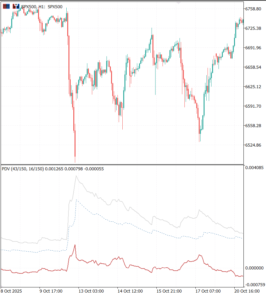
PDV decomposition on SPX500 H1 through the October 2025 crash and recovery

Fig. 4. SPX500 H1, October 2025. The trend term is strongly positive through the crash and negative through the recovery that follows, while activity stays elevated in both. The sign is the part a conditional-variance model cannot report separately.

In Fig. 4 the dotted activity line behaves like the EWMA volatility it essentially is, climbing into the 10 October crash and staying elevated through the recovery, indifferent to direction. The red trend line separates the two episodes. At the crash it reaches +9.29e-04 against an activity term of 1.934e-03, lifting total volatility to 3.386e-03, some 38% above activity plus baseline. In the rally off the 17 October low it falls to -3.27e-04 against an activity term of 1.249e-03, pulling the total down to 1.445e-03, some 18% below that same figure.

Between those bars the trend term swings by 1.256e-03 and activity by only 6.85e-04. In this episode the directional component moves nearly twice as far, across two stretches a single volatility number would call the same elevated regime; over the whole sample, though, the trend term is the smaller of the two, as section seven shows. Activity says how much, trend says which way, and only activity survives being squared.

Two features need reading correctly. b0 is the intercept, a constant offset of 5.2273e-04, not a floor, so the gap between the total and the activity line is b0 plus the trend term; read the trend from the red line, not the gap. The total usually sits above the activity line, but drops beneath it once the trend term falls below -b0, as at 23:00 on 27 October, when it reaches -5.42e-04. And the trend term does not collapse when a move ends: the fitted kernels weight a long memory heavily and still carry the crash days later, which is the model working as specified, not a lag to tune out.

Does It Beat GARCH?

PDV_Evidence answers this, and the method matters as much as the answer. Five models are compared on identical bars, target and chronological split, all fitted on the same purged training rows, and every baseline gets the same intercept and slope the model gets. Without that, the comparison would measure whether an EWMA happens to be quoted on the target's scale, not whether it carries the same information.

//+------------------------------------------------------------------+
//| Fit a raw proxy's affine map on the purged training rows         |
//| [first,fit_last], then score both halves.                        |
//+------------------------------------------------------------------+
double FitAndScore(const double &raw[],const double &y[],const int first,const int fit_last,
                   const int split,const int last,double &r2_train,double &r2_test,
                   double &rmse_test)
  {
   double c0,c1;
   r2_train =0.0;
   r2_test  =0.0;
   rmse_test=0.0;
   if(!AffineFit(raw,y,first,fit_last,c0,c1))
      return DBL_MAX;

   double pred[];
   ArrayResize(pred,last+1);
   ArrayInitialize(pred,0.0);
   for(int i=first;i<=last;i++)
      pred[i]=c0+c1*raw[i];

   double rm_train=0.0;
   r2_train=ScoreR2(pred,y,first,fit_last,rm_train);
   r2_test =ScoreR2(pred,y,split,last,rmse_test);

   double sse=0.0;
   for(int i=first;i<=fit_last;i++)
     {
      const double e=y[i]-pred[i];
      sse+=e*e;
     }
   return sse;
  }

The GARCH baseline gets the same care, and one alignment decision inside it separates a fair test from a rigged one:

//+------------------------------------------------------------------+
//| GARCH(1,1) conditional volatility under variance targeting.      |
//|                                                                  |
//|  Written to include bar i's own return, so it lines up with the  |
//|  PDV features rather than lagging them by one bar - otherwise    |
//|  the comparison would be handicapping GARCH by a bar of          |
//|  information rather than by its structure. Omega is pinned by    |
//|  variance targeting, which is standard practice and leaves the   |
//|  two coefficients that actually shape the response.              |
//+------------------------------------------------------------------+
void BuildGarch(const double &ret[],const int total,const double alpha,const double beta,
                const double uncond_var,double &out[])
  {
   const double omega=(1.0-alpha-beta)*uncond_var;
   double h=uncond_var;
   ArrayResize(out,total);
   out[0]=MathSqrt(h);
   for(int i=1;i<total;i++)
     {
      h=omega+alpha*ret[i]*ret[i]+beta*h;
      if(h<=0.0)
         h=uncond_var;
      out[i]=MathSqrt(h);
     }
  }

Stored at index i, the value is the variance for bar i+1 given the close of bar i, the textbook one-step-ahead forecast, and the target at bar i starts at bar i+1. The coefficients are searched over persistence and alpha rather than alpha and beta: intraday persistence sits above 0.98, where a grid uniform in beta has almost no resolution, and the baseline would lose to its own coarse search. The grid minimises the same squared error the table scores, which suits GARCH better than a likelihood fit would. The comparison is with GARCH(1,1); the asymmetric variants of section one are not in it.

Every figure here comes from one PDV_Evidence run: up to 40,000 H1 bars of whatever history the terminal held locally for each symbol, a Parkinson target 24 bars ahead, a 750-bar warm-up, a 70/30 chronological split, the EWMA searched over 40 half-lives and GARCH over a 22-by-22 grid in persistence and alpha. That history did not end on the same day everywhere: SPX500 (22,409 bars) and BTCUSD on 7 August 2026, the currency pairs and gold on 7 September 2026, the other indices in between. The split dates differ, so compare the models on a symbol, not the symbols. Here is SPX500:

Model	R-squared, train	R-squared, test	RMSE test	Fitted
constant	0.0000	-0.0233	6.9659e-04	mean 1.701e-03
EWMA volatility	0.5661	0.2666	5.8972e-04	half-life 16.4
GARCH(1,1)	0.5667	0.2693	5.8863e-04	alpha 0.039 beta 0.958
PDV, activity only	0.5676	0.2753	5.8621e-04	b2 0.7375
PDV, full	0.6539	0.4464	5.1237e-04	b1 -2.3949 b2 0.6837

Read the "PDV, activity only" and "PDV, full" rows together. The activity-only model, PDV without the trend term at its own optimum, scores 0.2753 out of sample, within 0.006 of GARCH: by themselves, two-exponential kernels and a careful fit buy almost nothing over GARCH(1,1). The full model scores 0.4464. The +0.171 difference is the value of adding the trend term, its four parameters and the readjustment of the activity side they permit; nothing else in the specification differs.

Across ten instruments the pattern is sharp:

Symbol	b1	Activity only	Full	R2 from trend	vs GARCH
SPX500	-2.3949	0.2753	0.4464	+0.1711	+0.1771
US30	-1.7569	0.2273	0.3857	+0.1584	+0.1557
NDX100	-1.5465	0.3401	0.4538	+0.1137	+0.1250
JP225	-1.8994	0.3547	0.4328	+0.0781	+0.0941
GER30	-0.8764	0.3686	0.4416	+0.0730	+0.1302
XAUUSD	+0.6608	0.5192	0.5419	+0.0226	+0.0281
BTCUSD	-0.1529	0.3583	0.3723	+0.0140	+0.0571
GBPUSD	-0.8774	0.2286	0.2396	+0.0110	+0.0433
USDJPY	-0.3393	0.3237	0.3329	+0.0092	+0.0123
EURUSD	-0.5051	0.3707	0.3637	-0.0070	+0.0205

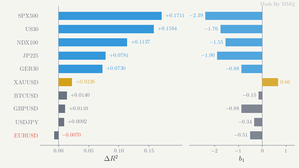
Out-of-sample R-squared added by the trend term across ten instruments

Fig. 5. What the sign of the path is worth, by instrument. The five equity indices separate cleanly from everything else.

Every equity index sits between +0.073 and +0.171; every currency pair within about a hundredth of zero, with EURUSD very slightly harmed. That is consistent with the usual explanations of the effect. The classic one is financial leverage: a falling share price raises a firm's debt-to-equity ratio and makes its equity riskier. The other, volatility feedback, has rising expected volatility pushing prices down. Both are about equity, with no obvious counterpart in a currency pair, which has no issuer whose balance sheet can be geared.

The currency rows say no more than that. GBPUSD's b1 of -0.877 matches GER30's -0.876; the coefficient is there in sample and does not carry out of sample. Currencies have their own asymmetries, such as risk-off flows into the yen, carry unwinds and intervention, whose sign depends on which side is the base currency, so one b1 per pair is a blunt tool. This specification finds nothing worth having on these pairs at this horizon and with this target; that does not prove currency volatility has no path dependence.

Gold's b1 is positive: rising prices go with rising volatility, which would fit an asset whose rallies are the stress events. Treat it as a hint. The gain is small, +0.023, and fragile: refitting the same history with the purged training window lands in a neighbouring optimum near +0.009, inside the currency band, and one instrument on one horizon cannot separate a mechanism from a feature of the period.

What the Numbers Do Not Say

Seven caveats. The first four we measured, the fifth concerns the forward projection, and the last two are about what was not measured.

A noisy target keeps R-squared well below 1. Realised volatility from a finite number of bars carries its own sampling noise, and no model explains noise. On synthetic data generated by the model with known parameters, the fit reaches an out-of-sample R-squared of 0.1156 against a close-to-close target, and a forecaster handed the true current volatility, rescaled to the target's mean, scores 0.1114. That is a benchmark, not a ceiling: it has no intercept and knows the current bar's volatility rather than the expected path over the target's 24 bars, so a fitted model can edge past it. It does show that a model at the right volatility scores only about 0.11 against such a target, so a low R-squared there is not by itself a failure. Against the true volatility the fit correlates at 0.976. The Parkinson target used elsewhere is far less noisy, hence the higher real-data figures. Read them against the baselines in section six, never against 1.0.

The kernel parameters are weakly identified. On the same test the calibrator recovered half-lives of 0.50 and 121.5 for a series generated with 4 and 60, with 98% of the weight on the 121.5-bar side, in effect one exponential, yet matched the fit of the true kernels and tracked the true volatility at 0.976. Very different kernels describe the same market almost equally well, so report the fitted curve and the decomposition, not the half-lives as structural constants. The 150-bar half-lives of section four describe that fit, not the market.

More memory stops paying out of sample. This sweep varies only the half-life cap. The warm-up is pinned at 3,500 bars for every row, what a 700-bar half-life needs and what SetMaxHalfLife would otherwise refuse, because raising it with the cap would move the scored window and credit the cap for a change of period. The window therefore starts 2,750 bars later than elsewhere, so these figures run higher than section four's and compare only with each other.

Cap	R-squared, train	R-squared, test	b1
50	0.6941	0.4446	-1.911
100	0.6991	0.4550	-2.134
150	0.7029	0.4575	-2.479
300	0.7080	0.4542	-3.843
500	0.7093	0.4523	-5.312
700	0.7095	0.4533	-5.939

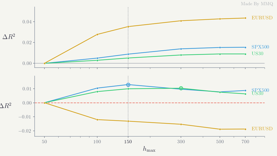
Train and test R-squared against the half-life cap on SPX500

Fig. 6. In-sample R-squared rises monotonically with memory while out-of-sample R-squared rises to about 150 bars and then flattens slightly lower.

Training R-squared rises monotonically. Out-of-sample R-squared climbs 0.013 from a 50-bar cap to 150, then sits 0.003 to 0.005 lower at every longer cap, not monotonically, and differences that small cannot be called without an interval. Meanwhile b1 inflates from -1.9 to -5.9 as it absorbs memory that does not generalise. A 750-bar warm-up, capping half-lives at 150, is a reasonable choice on H1 indices, not a proven optimum.

The model can produce a negative volatility. With b1 negative, a long enough rally drives b0 + b1 * R1 + b2 * sqrt(R2) through zero. That is a property of the linear specification, not a porting error, and it is handled in one helper, so the live reading and the multi-step forecast apply the same floor:

//+------------------------------------------------------------------+
//| Apply the floor: a share of the activity term's magnitude, so it |
//| carries the instrument's scale whatever the sign of b2.          |
//+------------------------------------------------------------------+
double CPdvForecast::Floored(const double raw,const double root) const
  {
   const double flr=m_floor_frac*MathAbs(m_p.b2)*root;
   if(flr<=0.0)
      return (raw>0.0 ? raw : 0.0);
   return (raw<flr ? flr : raw);
  }

The live reading is that helper applied to the raw value:

//+------------------------------------------------------------------+
//| Model volatility, floored.                                       |
//+------------------------------------------------------------------+
double CPdvForecast::Sigma(void) const
  {
   return Floored(SigmaRaw(),m_state.RootR2());
  }

Both values are exposed because the raw one is a diagnostic: it shows the model has been pushed outside the range it was fitted in. On SPX500 the floor never engaged over 22,120 described bars, so there the indicator runs exactly the calibrated model; on another instrument, check the negative-raw-sigma count PDV_Calibrate prints. As a share of the activity term's magnitude, the floor keeps its scale even if a fit returned a negative b2, itself a sign of an unusable fit.

On thresholds: the mean trend share on SPX500 is 0.168, and over those 22,120 bars the trend term never exceeded the activity term in magnitude. In bins a tenth wide, 29% of bars fall below 0.1, 34% between 0.1 and 0.2, 28% between 0.2 and 0.3, 10% between 0.3 and 0.4, and none above. A rule such as "act when the trend share passes one half" would never fire, although the trend term is worth 0.171 of R-squared. Thresholds are not useless, but one borrowed from intuition sits outside the range the quantity occupies; rank the trend share against its own recent distribution instead.

The multi-step forecast settles far more slowly than its half-life suggests. Projecting forward with no new information is where the separate UpdateParts promised in section three earns its keep:

//+------------------------------------------------------------------+
//| Volatility this many bars ahead, given no further information.   |
//|                                                                  |
//|  With nothing new arriving the expected return is zero, so the   |
//|  signed accumulators simply decay. The squared ones cannot decay |
//|  to zero, because the model's own answer is what the market is   |
//|  expected to deliver: each step feeds the current sigma squared  |
//|  back in as the next bar's squared return. The recursion relaxes |
//|  toward the model's fixed point, b0/(1-b2), rather than toward   |
//|  nothing - which is why a long-horizon forecast flattens out     |
//|  instead of collapsing. Note that the b2 feedback stretches the  |
//|  relaxation well beyond the kernel's own half-life.              |
//|                                                                  |
//|  Working on a copy keeps this a query, so a caller can forecast  |
//|  on every tick without disturbing the live reading.              |
//+------------------------------------------------------------------+
double CPdvForecast::Forecast(const int steps) const
  {
   if(!m_ready)
      return 0.0;
   if(steps<=0)
      return Sigma();

   CPdvState fwd;
   fwd.CopyFrom(m_state);
   double sig=Sigma();

   for(int k=0;k<steps;k++)
     {
      fwd.UpdateParts(0.0,sig*sig);
      const double root=fwd.RootR2();
      const double raw =m_p.b0+m_p.b1*fwd.R1()+m_p.b2*root;
      sig=Floored(raw,root);
     }
   return sig;
  }

The signed side is fed zero and the squared side the model's own answer, an asymmetry a single Update could not express. With b2 at 0.684 the fixed point b0 / (1 - b2) is about 1.65e-03 on SPX500, close to the unconditional mean in the evidence table, but the feedback stretches the approach far past the kernel's memory: a forecast built on a 40-bar half-life takes several hundred bars to settle, not forty. An answer stubbornly close to today's reading is that property of the specification, not a bug.

Not measured here: every out-of-sample number in this article scores the one-step feature set against a target 24 bars ahead. The multi-step projection is shipped and its behaviour understood, but it is not separately validated; treat it as a facility, not a benchmarked forecast.

None of these differences carries a confidence interval. The 24-bar targets overlap: the 6,629 scored SPX500 test bars hold only about 276 non-overlapping windows, and volatility persistence shrinks the effective sample further. The +0.17 on SPX500 is large against that; the currency differences of about a hundredth, gold's +0.023 and the cap sweep's thousandths are not distinguishable from noise without a formal test, such as Diebold-Mariano with autocorrelation-robust errors, which is not run here.

Every result comes from one setup: H1 bars, a 24-bar horizon, a Parkinson target, one 70/30 split, ten instruments, one broker's history. Nothing here shows the same holds on other timeframes, horizons, targets or data sources. GER30 is a warning: with one more month of history, every volatility model's out-of-sample R-squared on it, EWMA and GARCH included, falls from about 0.4 to about zero, while the gain from the trend term stays at +0.07 to +0.10. Levels are fragile; the comparison between models on one symbol is the sturdier reading.

Conclusion

We started from a structural complaint: a conditional-variance model reads past squared returns, and its asymmetric variants admit the sign only through the variance's own memory, never as a memory of the path's direction. We ported a model that has one, and measured what it is worth.

The implementation is four numbers. Two mixtures of two exponentials become four EWMA accumulators updated with eight multiplications per bar, with no lookback window, no matrix in the update and nothing that grows with history. Calibrating all nine parameters takes about 1.2 seconds on 22,000 bars.
The trend term is worth a great deal on equity indices. Against the same model without it, each fitted at its own optimum, it adds 0.073 to 0.171 of out-of-sample R-squared on all five indices tested, with 0.171 on SPX500 and 0.158 on US30 at the top, and it beats a fairly searched GARCH(1,1) by a similar margin on every one.
It adds nothing measurable on currency pairs. That fits the equity-based accounts of the leverage effect, but shows only that this specification finds nothing worth having at this horizon, not that currency volatility has no path dependence.
The decomposition is the deliverable, not the R-squared. Splitting volatility into direction and activity answers a question a single conditional-variance number cannot, at no extra cost.
Read the caveats. A noisy target keeps R-squared well below 1, the half-lives are weakly identified, memory beyond about 150 bars buys nothing out of sample, no difference carries a confidence interval, and every figure comes from one setup. The trend share never exceeds 0.4 on SPX500, so set thresholds from the observed distribution, not from intuition.

To reproduce this on your instrument, run PDV_Calibrate on the symbol and timeframe you trade. Check that b1 is far enough from zero to do work and keeps its sign when you move the end of the history by a few weeks, and that the negative-raw-sigma count is near zero. Paste the nine printed numbers into PDV_Decomposition, and run PDV_Evidence to confirm the trend term earns its place before you rely on it. If the activity-only and full rows land within a hundredth of each other, as on EURUSD, the extra term buys nothing on that instrument, and you should say so.

The programs presented in this article are intended for educational purposes only. Backtested and in-sample results do not guarantee future performance, and the models discussed here forecast volatility rather than direction. Nothing in this article is a recommendation to trade.

Getting the Source Code via MQL5 Algo Forge

All source files are attached to this article below, but the full repository is also available on MQL5 Algo Forge, the community's Git-based platform for sharing and collaborating on trading projects.

File name	Description
MQL5\Include\PDV\PdvTypes.mqh	Shared vocabulary: kernel, parameter, fit and decomposition structs, buffer map, half-life conversions
MQL5\Include\PDV\PdvState.mqh	The model engine: four exponential accumulators updated in O(1) per bar
MQL5\Include\PDV\PdvModel.mqh	Calibration: forward-only target construction, closed-form regression, Nelder-Mead over the kernels, activity-only ablation
MQL5\Include\PDV\PdvForecast.mqh	Live model: decomposition, volatility floor, trend share, multi-step projection
MQL5\Indicators\PDV\PDV_Decomposition.mq5	Subwindow indicator plotting total volatility against its trend and activity components
MQL5\Scripts\PDV\PDV_Calibrate.mq5	Fits the model to one symbol and reports parameters, split scores and the decomposition summary
MQL5\Scripts\PDV\PDV_Evidence.mq5	Out-of-sample comparison against a constant, an EWMA volatility and GARCH(1,1), with the trend-term ablation

Attached files |

Download ZIP

MQL5.zip (28.86 KB)

Warning: All rights to these materials are reserved by MetaQuotes Ltd. Copying or reprinting of these materials in whole or in part is prohibited.

This article was written by a user of the site and reflects their personal views. MetaQuotes Ltd is not responsible for the accuracy of the information presented, nor for any consequences resulting from the use of the solutions, strategies or recommendations described.