The Chimp Optimization Algorithm: From ChOA to BChimp
 159
 0

Contents
Introduction
Among population-based metaheuristics whose mechanisms are modeled on collective animal behavior, algorithms inspired by group hunting occupy a distinct niche. The best-known example — the Grey Wolf Optimizer (GWO) — is based on a simple hierarchy: the entire pack moves toward the three best individuals, and each wolf follows the same strategy. The Chimp Optimization Algorithm (ChOA), proposed by Khishe and Mosavi in 2020, superficially resembles this scheme but is based on a different idea — the heterogeneity of intelligence within the group.
Chimpanzees live in a fission-fusion society, where the composition and size of hunting groups are constantly changing, and where hunting success depends not on uniformity but on the division of roles. The authors of the algorithm identify four types of individuals with different abilities and strategies: drivers follow the prey and pressure it without attacking; barriers block escape routes, trapping the prey; chasers quickly catch up with the prey, causing panic; and, finally, attackers anticipate the escape route and finish the hunt. In optimization terms, these four roles are assigned to the four best solutions in the population, and the remaining individuals update their positions based on all four leaders at once, rather than on a single leader. It is precisely this heterogeneity — the different laws governing changes in coefficients for different groups — that distinguishes ChOA from the homogeneous GWO family.
The second pillar of the algorithm is what the authors refer to as social motivation. In addition to rational pursuit of prey, chimpanzees tend to exhibit impulsive, chaotic behavior — a drive to obtain meat at any cost for subsequent social exchange. In the mathematical model, this translates into a chaotic component: with a certain probability, an individual updates its position not according to the hunting formulas, but by a jump determined by a chaotic map. The purpose of this mechanism is to enable the algorithm to escape from local optima to which a smooth collective search inevitably converges.
Mathematically, ChOA can be described concisely. Each individual's position is recalculated as the average of four candidate positions. Each candidate is drawn toward its leader using a distance distorted by random and chaotic coefficients. The dynamic coefficient, which determines the balance between exploration and exploitation, decreases monotonically over the course of the iterations: at the beginning, the steps are large and the population explores the space extensively; by the end, it converges toward the leaders it has found. The chaotic replacement described above operates on top of this.
ChOA is, by its very nature, continuous. However, many applied problems require a binary solution. A classic example is feature selection in machine learning, where a subset must be chosen from thousands of features, and the solution is encoded as a bit string indicating included/excluded. In 2023, Ayeche and Alti closed this gap by proposing Enhanced Binary Chimp (BChimp): they took the ChOA core and added a binarization layer in two variants — BChimp1 (stochastic crossover of four binary steps) and BChimp2 (a sigmoid transfer function). It is this work that we use as our basis — the specific coefficient curves and the algorithm's formulation itself are taken from it.
However, our ranking covers continuous optimization, so we remove the binarization layer, revealing the same continuous core beneath it — in terms of its mechanism, this corresponds to the original ChOA, bringing us full circle. Naming convention in this article: we retain the name BChimp for the implementation, after the specific work we reproduce and test, and use ChOA when referring to the continuous predecessor that provided the core.
In this article, we will implement the algorithm using the standard C_AO framework. We will run it through the usual set of test functions (Hilly, Forest, Megacity) at different dimensionalities and assess its position in the shared ranking. Along the way, we'll need to carefully compare the code with the publication and the original source. We will also need to correct an inherited coefficient defect that goes unnoticed in a binary problem but destroys the search in a continuous one — and, in the process, uncover hidden characteristics of the algorithm that distort its evaluation on the usual tests.
Implementation of the Algorithm
Population structure and the quartet of leaders. The ChOA population consists of NN chimpanzees, each of which is a solution point in the search space. At each iteration, the four individuals with the highest fitness are designated as leaders and assigned the roles of Attacker, Barrier, Chaser, and Driver. This group of four conveys information about the most likely location of the prey; the remaining members adjust their positions, using all four leaders as reference points.
Basic hunting equations. An individual's approach to the prey is described by two vector equations. First, the distance between the individual and the target being pursued is calculated:
Then, the new position is calculated from this distance:
Here, is the individual’s current position, is the leader’s position, and , and are coefficients that govern behavior. The coefficient determines the magnitude and direction of the step; determines the weight of the leader’s position in the distance calculation; is a chaotic multiplier modeling impulsivity.
Dynamic coefficients. The coefficients a and c are constructed from a decreasing control parameter f and random numbers:
where is the current iteration number, is the total number of iterations, and . Parameter decreases linearly from 2 to 0: at the beginning of the run may exceed one, and the agent takes large steps (exploration); by the end and the steps converge toward the leaders (exploitation).
The diversity of the four roles stems from the fact that for each group and are scaled by their respective dynamic curves. For the four groups:
Two groups use the cube-root law , producing a rapid initial decrease followed by a gently sloping tail; the other two use the cubic law , which, conversely, keeps the value high for a long time before it drops sharply at the end. Thus, the groups achieve different balances between exploration and exploitation over time. (Note: In the authors’ reference code, the curves and are expressed using the cubic law rather than the cube-root law given in the article — a minor discrepancy that we will return to later.)
Four-leader position update. Each individual computes four candidate positions — one for each leader. For the attacker:
and similarly for the barrier, chaser, and driver, each with their own coefficients , . The final position is the average of the four candidate positions:
Averaging is the mechanism that pulls the population toward the best solutions: each individual ends up at the center of gravity of four attractive forces.
The chaotic component and social motivation. The second pillar of the algorithm is chaotic behavior, which reflects the chimpanzee’s impulsive drive to capture prey. With a 50% probability, the regular four-leader position update is replaced by a jump determined by a chaotic map:
where is a random number. A chaotic value is generated by one of the deterministic maps — the logistic map, Gauss map, tent map, etc. The logistic map, for example, is iterated as
and, for an initial value that is not a fixed point, yields an aperiodic sequence in . The purpose of this phase is to give the population ways to escape local optima that smooth collective movement alone cannot provide.
Binarization: BChimp1 and BChimp2. ChOA itself is continuous. For problems where the solution is a bit string (feature selection), Ayeche and Alti added a binarization layer to the ChOA core in two variants.
BChimp1 converts each of the four candidates into a binary step. First, the continuous step is passed through a sigmoid function:
The result is then compared with a random number to produce a binary step, which is added to the leader's position:
From the four binary vectors Y1,…,Y4, the final coordinate is chosen at random — stochastic crossover with an equal probability of for each vector.
BChimp2 takes a different approach: it averages four continuous candidates and passes the average through a sigmoid function with a threshold cutoff:
In both cases, continuous values are not stored anywhere — they instantly collapse to 0 or 1. This is an important point: binarization masks any scale and sign characteristics of the continuous step. It is precisely this feature that hides the flaw we are about to examine.
Example: Coefficient bias in A. Let's construct the coefficient as specified in the publication. The control parameter remains shared, while the group-specific curve is incorporated into the random factor: . Substituting gives:
Let's calculate the expected value. Since with a mean of :
At the start of the run, and , so
The coefficient is, on average, positive and large. The update has the form , where . Positive systematically shifts the coordinate below that of the leader — and does so along all axes simultaneously, since the coefficient structure is the same for all coordinates. The result is a directed drift of the entire population toward the corner of the search space and movement along the main diagonal. Toward the middle of the run, decreases, changes sign, and the population is driven back out of the corner: this is not convergence, but oscillation caused by coefficient bias.
In a binary problem, this is not apparent: whatever the value of the continuous product , the sigmoid and threshold convert it to 0 or 1. But as soon as you remove the binarization, the algorithm performs worse than a random search.
This can be corrected by symmetrizing the random part. Instead of the shifted factor , we use the symmetric factor with zero mean; retaining the shared factor , we obtain
Now the coefficient is symmetric about zero — on average, the individual does not move toward or away from the leader — and the amplitude decays to zero by the end of the run, ensuring convergence. (In canonical ChOA, the same symmetry is achieved even more simply: the group curve itself serves as the amplitude , and is uniform.) This is precisely the form we use in our implementation; the next section discusses it and the results.
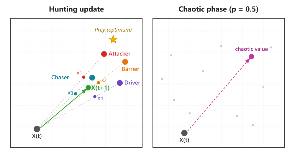
Figure 1. Two Position Update Modes in ChOA
The left panel shows the hunting phase. Individual X(t) (gray) repositions itself using the four leaders surrounding the prey as reference points: the attacker, the barrier, the chaser, and the driver. For each leader, a candidate (X1…X4) is calculated — an attraction along the corresponding direction with its own role coefficients. The new position X(t+1) (green) is the average of the four candidates — the center of gravity of the attractions, pulling the population toward the best solutions.
The right panel shows the chaotic phase. With a probability of 0.5, a regular update is replaced by a jump: the individual’s coordinates are replaced by the value of a chaotic map (the gray dots show how the chaotic sequence covers the search space). It is precisely this phase that has been omitted from our continuous implementation.
Below is the pseudocode for BChimp as implemented and tested for the ranking: a continuous ChOA core with a corrected coefficient a, without the chaotic replacement phase.
Input:  N — population size, T — number of iterations, [lo, hi] — search bounds
Output: best found solution

 1.  Randomly initialize population X = {X_1, …, X_N} into [lo, hi]
 2.  Set static chaotic multiplier m[i] for each agent
         (Piecewise map, one value per agent, calculated only once)
 3.  Calculate the fitness of all agents
 4.  Select four leaders based on fitness:
         X_attacker, X_barrier, X_chaser, X_driver

 5.  for t = 1 … T:

 6.      f = 2 − 2·(t/T)                              // shared factor, 2 → 0
 7.      // group curves, k = 1–4
 8.      C1G_1 = C1G_2 = 1.95 − 2·(t/T)^(1/3)
 9.      C1G_3 = C1G_4 = −2·(t/T)^3 + 2.5
10.      C2G_1 = C2G_3 = 2·(t/T)^(1/3) + 0.5
11.      C2G_2 = C2G_4 = 2·(t/T)^3     + 0.5

12.      for each agent i:
13.          for each coordinate j:
14.              sum ← 0
15.              for each leader k ∈ {attacker, barrier, chaser, driver}:
16.                  a_k = f · C1G_k · (2·rand() − 1)           // symmetric, E[a] = 0
17.                  c_k = C2G_k · rand()
18.                  d_k = | c_k · X_leader_k[j] − m[i] · X_i[j] |
19.                  sum += X_leader_k[j] − a_k · d_k
20.              X_i[j] ← sum / 4
21.              clamp X_i[j] to [lo[j], hi[j]]

22.      Calculate the fitness of all agents
23.      Update the four leaders (elitist update: retain the four best solutions found so far)
24.      Update the global best

25.  return the global best
Coordinate-wise randomness. The coefficients a_k and c_k are resampled for each coordinate j; each agent has its own chaotic multiplier m[i]. Even though m[i] is the same for all of the agent’s coordinates, the coordinate-wise variation is provided by a_k and c_k — therefore, a shared scalar that confines a candidate to a subspace does not arise, and there is no diagonal advantage on a symmetric benchmark.
Symmetric a. The factor f·C1G_k specifies the step amplitude and decays to zero by the end of the run, while the factor (2·rand − 1) makes the step symmetric (mean zero). This corrects the defect discussed in the description section: in the published form, the random component is shifted away from zero, causing the population to drift into a corner in continuous search.
Elitism. Each of the four leaders stores its best-ever position, rather than the best position in the current population; the population itself moves freely, without rollback.
The chaotic replacement phase of the original ChOA (where a position is replaced by a chaotic value with a probability of 0.5) has been omitted: in the continuous problem, it proved to be detrimental to convergence. For a binary problem (feature selection), line 20 is replaced by a binarization step — either sigmoid thresholding of the mean (BChimp2) or crossover of four binary steps (BChimp1).
Let's move on to the implementation. The C_AO_BChimp class inherits from the base class C_AO and follows the framework's standard life cycle: the Moving method proposes new positions, the outer loop evaluates fitness, and the Revision method updates the best positions. All internal state beyond that of the base agent is stored in structures — this keeps the data for the four leaders and the individual state of each agent self-contained, without flat buffers (index × coordinate).
The four leaders are stored as an array called lead[4] (0 = attacker, 1 = barrier, 2 = chaser, 3 = driver). Each leader is self-contained, and working with it does not require manually recalculating offsets in the shared buffer. In addition, the class maintains the iteration counters epochs, epochsDen, and epochNow for the t/T ratio, as well as a single visible parameter, popSize.
//+------------------------------------------------------------------+
class C_AO_BChimp : public C_AO
 {
public:
                    ~C_AO_BChimp() {}
                     C_AO_BChimp()
   {
    ao_name = "BChimp";
    ao_desc = "Chimp Optimization Algorithm";
    ao_link = "https://www.mql5.com/en/articles/23132";

    popSize = 30;

    ArrayResize(params, 1);
    params [0].name = "popSize";
    params [0].val  = popSize;
   }

  void               SetParams()
   {
    popSize = (int)params [0].val;
   }

  bool               Init(const double &rangeMinP  [],
                          const double &rangeMaxP  [],
                          const double &rangeStepP [],
                          const int     epochsP = 0);

  void               Moving();
  void               Revision();

private:
  //--- four leaders: 0=attacker, 1=barrier, 2=chaser, 3=driver
  S_Leader           lead [4];

  //--- agents' individual state
  S_Chimp            chimp [];

  //--- iteration counters (for the ratio t/T)
  int                epochs;
  int                epochsDen;
  int                epochNow;

  //--- attempt to insert an agent into the elite leader ranking
  void               InsertLeader(const int i);
 };
The pack leader is described by the S_Leader structure — coordinates and fitness in a single object:
//+------------------------------------------------------------------+
//| Pack leader: coordinates + fitness                               |
//+------------------------------------------------------------------+
struct S_Leader
 {
  double c           [];   // coordinates
  double             f;      // fitness

  void               Init(const int coords)
   {
    ArrayResize(c, coords);
    f = -DBL_MAX;
   }
 };
The individual state of an agent is represented by the S_Chimp structure with a single field, m, the chaotic multiplier. There is only one field, but moving it into the structure separates the algorithm's state from the base S_AO_Agent and leaves room for expansion.
//+------------------------------------------------------------------+
//| Individual state of a chimpanzee                                 |
//+------------------------------------------------------------------+
struct S_Chimp
 {
  double             m;      // chaotic multiplier (Piecewise map), static
 };
Init begins with StandardInit, which sets up the search boundaries and the array of agents. The initial population is then randomly distributed into cP[] — on the first call to Moving, it will be copied to the working coordinates c[] so that the outer loop can evaluate it. The four leaders are initialized with a fitness of -DBL_MAX, representing empty slots that will be filled during the first revision.
A separate block precomputes the chaotic multiplier based on the Piecewise map (index 6, P = 0.4, initial value x0 = 0.7). The value is taken before the next map update. Each agent receives its own static multiplier m[i], which is the same for all its coordinates and remains unchanged throughout the run — exactly as in the original implementation. The epochsDen counter is set to epochs − 1: this ensures that the ratio t/T reaches one precisely on the last actual iteration, and the control multiplier f = 2 − 2·t/T correctly decays to zero by the end of the run.
//+------------------------------------------------------------------+
//|                              Init                                |
//+------------------------------------------------------------------+
bool C_AO_BChimp::Init(const double &rangeMinP  [],
                       const double &rangeMaxP  [],
                       const double &rangeStepP [],
                       const int     epochsP = 0)
 {
  if(!StandardInit(rangeMinP, rangeMaxP, rangeStepP))
    return false;

//--- initial random population in cP[] (will be copied to c[] on the first call to Moving)
  for(int i = 0; i < popSize; i++)
    for(int c = 0; c < coords; c++)
      a [i].cP [c] = u.RNDfromCI(rangeMin [c], rangeMax [c]);

//--- leaders
  for(int k = 0; k < 4; k++)
    lead [k].Init(coords);

//--- individual state
  ArrayResize(chimp, popSize);

//--- chaotic multiplier m[i] — Piecewise map (index=6 in the source),
//    P=0.4, x0=0.7, Value=1; the value is taken BEFORE the update
  double P = 0.4;
  double x = 0.7;
  for(int i = 0; i < popSize; i++)
   {
    chimp [i].m = x;
    if(x >= 0.0 && x < P)
      x = x / P;
    else
      if(x >= P && x < 0.5)
        x = (x - P) / (0.5 - P);
      else
        if(x >= 0.5 && x < 1.0 - P)
          x = (1.0 - P - x) / (0.5 - P);
        else
          x = (1.0 - x) / P;
   }

//--- iteration counters
  epochs    = epochsP;
  epochsDen = (epochs > 1) ? epochs - 1 : 1;
  epochNow  = 0;

  return true;
 }
The first call is special: while 'revision' is still 'false', the method simply transfers the starting coordinates from cP[] to c[] using the SeInDiSp projection (clamping to the boundaries while accounting for the step size) and exits, handing control back to the outer loop for the first evaluation.
On subsequent iterations, the epoch coefficients are recalculated first: the ratio tRatio = epochNow / epochsDen, the shared multiplier aCoef = 2 − 2·tRatio, and the group curves using the cube-root law u1 = (t/T)^{1/3} and the cubic law u3 = (t/T)^3 (arrays C1G, C2G). Next, for each agent and each coordinate, four candidates are generated — one per leader — and averaged.
The key detail is the form of Ak: the group curve C1G[k] serves as the amplitude, while randomness is introduced through a symmetric multiplier (2·rand − 1) with zero mean. This is precisely what corrects the inherited bias: in the published formulation, the random component was shifted, causing the population to drift toward a corner in continuous search space. Random values of Ak and Ck are drawn anew for each coordinate, so despite the scalar m[i], there is no shared multiplier for the entire vector, and the algorithm gains no geometric diagonal advantage.
//+------------------------------------------------------------------------+
//|                            Moving                                      |
//|                                                                        |
//|  1. First pass: cP -> c (the outer loop will evaluate FF);             |
//|  2. Next: a and four sets of coefficients per iteration;               |
//|  3. For each agent/coordinate—four candidates derived from the leaders,|
//|     averaging, projection into the bounds (SeInDiSp).                  |
//+------------------------------------------------------------------------+
void C_AO_BChimp::Moving()
 {
//--- first pass: cP -> c
  if(!revision)
   {
    for(int i = 0; i < popSize; i++)
      for(int c = 0; c < coords; c++)
        a [i].c [c] = u.SeInDiSp(a [i].cP [c], rangeMin [c], rangeMax [c], rangeStep [c]);
    return;
   }

//--- ratio t/T (clamped at 1.0); a: decay from 2 to 0
  epochNow++;
  double tRatio = (double)epochNow / (double)epochsDen;
  if(tRatio > 1.0)
    tRatio = 1.0;

  double aCoef = 2.0 - 2.0 * tRatio;

//--- dynamic group coefficients
//    u1 = (t/T)^(1/3) — cube-root law,  u3 = (t/T)^3 — cubic law
  double u1 = MathPow(tRatio, 1.0 / 3.0);
  double u3 = tRatio * tRatio * tRatio;

  double C1G [4], C2G [4];
  C1G [0] = 1.95 - 2.0 * u1;
  C2G [0] = 2.0 * u1 + 0.5;   // Group 1 (attacker)
  C1G [1] = 1.95 - 2.0 * u1;
  C2G [1] = 2.0 * u3 + 0.5;   // Group 2 (barrier)
  C1G [2] = -2.0 * u3 + 2.5;
  C2G [2] = 2.0 * u1 + 0.5;   // Group 3 (chaser)
  C1G [3] = -2.0 * u3 + 2.5;
  C2G [3] = 2.0 * u3 + 0.5;   // Group 4 (driver)

//--- movement
  for(int i = 0; i < popSize; i++)
   {
    double mi = chimp [i].m;

    for(int c = 0; c < coords; c++)
     {
      double xi  = a [i].c [c];
      double sum = 0.0;

      for(int k = 0; k < 4; k++)
       {
        //--- A is symmetric about 0: amplitude aCoef*C1G[k] → 0
        //    by the end of the run (E[A] = 0; no drift toward the corner). C is scaled
        //    to the canonical range [0..~2.5]. The sign of C1G[k] does not matter—it is multiplied
        //    by the symmetric term (2r-1).
        double Ak = aCoef * C1G [k] * (2.0 * u.RNDprobab() - 1.0);
        double Ck = C2G [k] * u.RNDprobab();
        double Dk = MathAbs(Ck * lead [k].c [c] - mi * xi);
        sum += lead [k].c [c] - Ak * Dk;
       }

      double v = sum / 4.0;
      a [i].c [c] = u.SeInDiSp (v, rangeMin [c], rangeMax [c], rangeStep [c]);
     }
   }
 }
Revision first updates the personal (fB, cB for each agent) and global (fB, cB) best solutions. Next, InsertLeader is called for each agent to maintain an elite group of four leaders: on the first call, the group is populated with the best individuals from the initial population; on subsequent calls, it is updated if an individual better than the current leaders is found. Leaders store the best positions found throughout the run, not the best positions in the current population.
There is no rollback (greedy acceptance) here — the population moves freely, and this is a deliberate choice: this is the reference version, with no additions on top of the original mechanics.
//+--------------------------------------------------------------------------+
//|                           Revision                                       |
//|                                                                          |
//|  Personal/global best updates + elitist update of the                    |
//|  four leaders (best-ever). No rollbacks—this is the reference version.   |
//+--------------------------------------------------------------------------+
void C_AO_BChimp::Revision()
 {
//--- update personal and global bests
  for(int i = 0; i < popSize; i++)
   {
    if(a [i].f > a [i].fB)
     {
      a [i].fB = a [i].f;
      ArrayCopy(a [i].cB, a [i].c, 0, 0, coords);
     }
    if(a [i].f > fB)
     {
      fB = a [i].f;
      ArrayCopy(cB, a [i].c, 0, 0, coords);
     }
   }

//--- elitist update of leaders (initialization on the first call
//    and maintenance of the top four on subsequent calls)
  for(int i = 0; i < popSize; i++)
    InsertLeader(i);

  if(!revision)
    revision = true;
 }
InsertLeader inserts an agent into a list of four leaders sorted in descending order of fitness. If an agent's fitness exceeds that of any of the leaders, the position found determines the insertion point, the tail of the list shifts downward, and the agent takes its place. Since the leaders are not reset between iterations, the set of four solutions accumulated in this way always reflects the four best solutions encountered since the start of the run.
//+---------------------------------------------------------------------------+
//|        InsertLeader — insert an agent into the leader list                |
//|  Leaders are sorted in descending order of fitness (lead[0] is the best). |
//+---------------------------------------------------------------------------+
void C_AO_BChimp::InsertLeader(const int i)
 {
  double f = a [i].f;

  int p = -1;
  if(f > lead [0].f)
    p = 0;
  else
    if(f > lead [1].f)
      p = 1;
    else
      if(f > lead [2].f)
        p = 2;
      else
        if(f > lead [3].f)
          p = 3;

  if(p < 0)
    return;

//--- shift downward from the tail to the insertion point
  for(int s = 3; s > p; s--)
   {
    lead [s].f = lead [s - 1].f;
    ArrayCopy(lead [s].c, lead [s - 1].c, 0, 0, coords);
   }

//--- insert
  lead [p].f = f;
  ArrayCopy(lead [p].c, a [i].c, 0, 0, coords);
 }
Test Results
On the full standard test suite, BChimp scored 33.94%, a typical result for most of the metaheuristics studied that did not make it into the ranking table.
BChimp|Chimp Optimization Algorithm|30.0|
=============================
5 Hilly's; Func runs: 10000; result: 0.6320626505708679
25 Hilly's; Func runs: 10000; result: 0.4688540395277016
500 Hilly's; Func runs: 10000; result: 0.25059324375826325
=============================
5 Forest's; Func runs: 10000; result: 0.45946276339630393
25 Forest's; Func runs: 10000; result: 0.19717796572435656
500 Forest's; Func runs: 10000; result: 0.054934191314905144
=============================
5 Megacity's; Func runs: 10000; result: 0.6186666666666667
25 Megacity's; Func runs: 10000; result: 0.27653333333333335
500 Megacity's; Func runs: 10000; result: 0.09597333333333409
=============================
All score: 3.05426 (33.94%)
The composite anti-cheat test provides a fair assessment:
BChimp|Chimp Optimization Algorithm|30.0|
=============================
Composite anti-cheat test: Hilly + Forest + Megacity + Peaks + Skin
Coordinates: 10; Epochs: 333; Repeats: 10
=============================
Run 1/10: 0.7950338893702603
Run 2/10: 0.7018012473036442
Run 3/10: 0.632016537203568
Run 4/10: 0.6372459064975272
Run 5/10: 0.605584348691656
Run 6/10: 0.7925826976716779
Run 7/10: 0.7760618579627041
Run 8/10: 0.6940213206471844
Run 9/10: 0.6152242781717281
Run 10/10: 0.8067332465317811
=============================
Average result: 0.7056305330 (70.56%)
=============================
Visualization of the BChimp algorithm running on the test suite and on several other functions.

BChimp on the Hilly test function

BChimp on the Forest test function

BChimp on the Megacity test function

BChimp on the Ackley test function

BChimp on the Shaffer test function
Based on the test results, the algorithm is included for informational purposes in the ranking of the best population-based optimization methods.
cc | AO | Description | Hilly | Hilly Final | Forest | Forest Final | Megacity (discrete) | Megacity Final | Final Result | % of MAX | ||||||
| 10 p (5 F) | 50 p (25 F) | 1,000 p (500 F) | 10 p (5 F) | 50 p (25 F) | 1,000 p (500 F) | 10 p (5 F) | 50 p (25 F) | 1,000 p (500 F) | ||||||||
| 1 | ANS | across neighbourhood search | 1.00000 | 0.88228 | 0.40138 | 2.28366 | 1.00000 | 0.95281 | 0.28092 | 2.23373 | 0.94667 | 0.85733 | 0.22389 | 2.02789 | 6.545 | 72.72 |
| 2 | AMOm | animal migration optimization M | 0.91624 | 0.83603 | 0.46790 | 2.22017 | 0.98482 | 0.92010 | 0.36391 | 2.26883 | 0.91733 | 0.81707 | 0.25177 | 1.98617 | 6.475 | 71.94 |
| 3 | CLA | code lock algorithm (joo) | 0.95139 | 0.86199 | 0.37879 | 2.19217 | 0.99349 | 0.93500 | 0.26497 | 2.19346 | 0.93600 | 0.84267 | 0.24060 | 2.01927 | 6.405 | 71.17 |
| 4 | (P+O)ES | (P+O) evolution strategies | 0.86571 | 0.89539 | 0.39740 | 2.15850 | 0.97761 | 0.89820 | 0.26878 | 2.14459 | 0.92133 | 0.80240 | 0.23952 | 1.96325 | 6.266 | 69.62 |
| 5 | SDSm | stochastic diffusion search M | 0.95195 | 0.84944 | 0.36249 | 2.16388 | 0.98061 | 0.88457 | 0.22112 | 2.08630 | 0.92267 | 0.79013 | 0.21380 | 1.92660 | 6.177 | 68.63 |
| 6 | AAm | archery algorithm M | 0.84685 | 0.73320 | 0.42590 | 2.00595 | 0.96709 | 0.77837 | 0.27789 | 2.02335 | 0.86133 | 0.77707 | 0.28712 | 1.92552 | 5.955 | 66.17 |
| 7 | SIA | simulated isotropic annealing (joo) | 0.93543 | 0.86504 | 0.38483 | 2.18530 | 0.94069 | 0.80609 | 0.23835 | 1.98513 | 0.86400 | 0.66160 | 0.19536 | 1.72096 | 5.891 | 65.46 |
| 8 | TETA | time evolution travel algorithm (joo) | 0.91452 | 0.86369 | 0.25579 | 2.03400 | 0.99654 | 0.91291 | 0.14394 | 2.05339 | 0.85467 | 0.82213 | 0.10443 | 1.78123 | 5.869 | 65.21 |
| 9 | ESG | evolution of social groups (joo) | 0.98111 | 0.79857 | 0.31167 | 2.09135 | 0.98954 | 0.82270 | 0.15032 | 1.96256 | 0.92133 | 0.73440 | 0.15315 | 1.80888 | 5.863 | 65.14 |
| 10 | CTA | comet tail algorithm (joo) | 0.92435 | 0.86786 | 0.27838 | 2.07059 | 0.99039 | 0.84571 | 0.19448 | 2.03058 | 0.95467 | 0.69680 | 0.11008 | 1.76155 | 5.863 | 65.14 |
| 11 | COA | coyote_optimization_algorithm | 0.88909 | 0.70681 | 0.32718 | 1.92308 | 0.99467 | 0.85358 | 0.15152 | 1.99977 | 0.88533 | 0.71040 | 0.18981 | 1.78554 | 5.708 | 63.43 |
| 12 | ECBO | enhanced colliding bodies optimization | 0.94024 | 0.72363 | 0.32356 | 1.98743 | 0.99477 | 0.80291 | 0.13056 | 1.92824 | 0.87600 | 0.70160 | 0.17433 | 1.75193 | 5.668 | 62.98 |
| 13 | DA | dialectical algorithm | 0.93117 | 0.75400 | 0.26205 | 1.94722 | 0.98925 | 0.81375 | 0.08662 | 1.88962 | 0.92667 | 0.68107 | 0.11315 | 1.72089 | 5.558 | 61.76 |
| 14 | BBO | biogeography-based optimization | 0.95876 | 0.70609 | 0.35752 | 2.02237 | 0.92981 | 0.70660 | 0.16970 | 1.80611 | 0.87467 | 0.63013 | 0.20813 | 1.71293 | 5.541 | 61.57 |
| 15 | BHAm | black hole algorithm M | 0.79558 | 0.76207 | 0.34682 | 1.90447 | 0.99836 | 0.75798 | 0.13826 | 1.89460 | 0.85067 | 0.64427 | 0.17020 | 1.66514 | 5.464 | 60.71 |
| 16 | HS | harmony search | 0.91420 | 0.69049 | 0.29924 | 1.90393 | 0.97627 | 0.73373 | 0.14193 | 1.85193 | 0.91733 | 0.62720 | 0.15364 | 1.69817 | 5.454 | 60.60 |
| 17 | RFO | royal flush optimization (joo) | 0.80989 | 0.74481 | 0.34546 | 1.90016 | 0.95251 | 0.77926 | 0.15185 | 1.88362 | 0.80400 | 0.66427 | 0.19071 | 1.65898 | 5.443 | 60.48 |
| 18 | BOAm | billiards optimization algorithm M | 0.76177 | 0.72421 | 0.25275 | 1.73873 | 0.90890 | 0.81960 | 0.28853 | 2.01703 | 0.83733 | 0.74613 | 0.09763 | 1.68109 | 5.437 | 60.41 |
| 19 | ASO | anarchy society optimization | 0.73070 | 0.73713 | 0.31195 | 1.77978 | 0.99732 | 0.87700 | 0.17619 | 2.05051 | 0.72000 | 0.68773 | 0.18988 | 1.59761 | 5.428 | 60.31 |
| 20 | EOm | extremal optimization_M | 0.76527 | 0.75205 | 0.31908 | 1.83640 | 0.99999 | 0.76426 | 0.12437 | 1.88862 | 0.84133 | 0.64133 | 0.15247 | 1.63513 | 5.360 | 59.56 |
| 21 | ACS | artificial cooperative search | 0.75545 | 0.77162 | 0.31653 | 1.84360 | 1.00000 | 0.80488 | 0.10705 | 1.91193 | 0.76933 | 0.60800 | 0.14157 | 1.51890 | 5.274 | 58.60 |
| 22 | SSG | saplings sowing and growing | 0.75436 | 0.63206 | 0.35935 | 1.74577 | 0.91907 | 0.69694 | 0.19755 | 1.81356 | 0.81867 | 0.60533 | 0.21347 | 1.63747 | 5.197 | 57.74 |
| 23 | AOSm | atomic orbital search M | 0.76184 | 0.68435 | 0.31344 | 1.75963 | 0.90015 | 0.80044 | 0.11501 | 1.81560 | 0.82800 | 0.63280 | 0.15696 | 1.61776 | 5.193 | 57.70 |
| 24 | TSEA | turtle shell evolution algorithm (joo) | 0.95809 | 0.64852 | 0.29571 | 1.90232 | 0.99522 | 0.58104 | 0.10542 | 1.68168 | 0.92133 | 0.52160 | 0.14567 | 1.58860 | 5.173 | 57.48 |
| 25 | DE | differential evolution | 0.96398 | 0.62346 | 0.26089 | 1.84833 | 0.98482 | 0.77018 | 0.11459 | 1.86959 | 0.93067 | 0.36213 | 0.11000 | 1.40280 | 5.121 | 56.90 |
| 26 | BIO | blood inheritance optimization (joo) | 0.72580 | 0.66522 | 0.31228 | 1.70330 | 0.99995 | 0.68125 | 0.11540 | 1.79660 | 0.85467 | 0.59333 | 0.15364 | 1.60164 | 5.102 | 56.69 |
| 27 | (PO)ES | (PO) evolution strategies | 0.73972 | 0.58190 | 0.38896 | 1.71058 | 0.91199 | 0.59975 | 0.21262 | 1.72436 | 0.82400 | 0.56240 | 0.23432 | 1.62072 | 5.056 | 56.18 |
| 28 | BO | bonobo optimizer | 0.75555 | 0.64366 | 0.32657 | 1.72578 | 0.94332 | 0.70442 | 0.13999 | 1.78773 | 0.73467 | 0.61440 | 0.16728 | 1.51635 | 5.030 | 55.89 |
| 29 | SRA | successful restaurateur algorithm (joo) | 0.89010 | 0.63359 | 0.29115 | 1.81484 | 0.96634 | 0.55285 | 0.08914 | 1.60833 | 0.89333 | 0.52800 | 0.13911 | 1.56044 | 4.984 | 55.38 |
| 30 | CRO | chemical reaction optimisation | 0.91281 | 0.65681 | 0.29866 | 1.86828 | 0.90513 | 0.56020 | 0.10939 | 1.57472 | 0.82800 | 0.50133 | 0.14149 | 1.47082 | 4.914 | 54.60 |
| 31 | BCOm | bacterial chemotaxis optimization M | 0.82589 | 0.61733 | 0.31584 | 1.75906 | 0.95296 | 0.63718 | 0.11984 | 1.70998 | 0.76533 | 0.51653 | 0.15800 | 1.43986 | 4.909 | 54.54 |
| 32 | DOA | dream optimization algorithm | 0.78522 | 0.78121 | 0.36036 | 1.92679 | 0.61584 | 0.42117 | 0.12254 | 1.15955 | 0.86667 | 0.72587 | 0.21127 | 1.80381 | 4.890 | 54.33 |
| 33 | ABO | african buffalo optimization | 0.92295 | 0.62528 | 0.29885 | 1.84708 | 0.92992 | 0.57468 | 0.09372 | 1.59832 | 0.73333 | 0.51333 | 0.14324 | 1.38990 | 4.835 | 53.72 |
| 34 | BSA | bird swarm algorithm | 0.94432 | 0.67941 | 0.26401 | 1.88774 | 0.91649 | 0.65619 | 0.12054 | 1.69322 | 0.80933 | 0.33547 | 0.10652 | 1.25132 | 4.832 | 53.69 |
| 35 | TSm | tabu search M | 0.87806 | 0.61040 | 0.28993 | 1.77839 | 0.98116 | 0.52165 | 0.08544 | 1.58825 | 0.82667 | 0.49547 | 0.13552 | 1.45766 | 4.824 | 53.60 |
| 36 | BSA | backtracking search algorithm | 0.87128 | 0.53190 | 0.28675 | 1.68993 | 0.92408 | 0.51602 | 0.09153 | 1.53163 | 0.96000 | 0.47253 | 0.13760 | 1.57013 | 4.792 | 53.24 |
| 37 | BWOm | beluga_whale_optimization_M | 0.78488 | 0.56872 | 0.29557 | 1.64917 | 0.91370 | 0.61760 | 0.12988 | 1.66118 | 0.81333 | 0.49946 | 0.15004 | 1.46283 | 4.773 | 53.04 |
| 38 | WOAm | whale optimization algorithm M | 0.93893 | 0.59477 | 0.26695 | 1.80065 | 0.98036 | 0.53873 | 0.07112 | 1.59021 | 0.78667 | 0.47600 | 0.11892 | 1.38159 | 4.772 | 53.02 |
| 39 | ACA | andean_condor_algorithm | 0.78444 | 0.53260 | 0.33108 | 1.64812 | 0.79071 | 0.44960 | 0.10685 | 1.34716 | 0.92266 | 0.67733 | 0.17613 | 1.77612 | 4.771 | 53.02 |
| 40 | CSO | competitive swarm optimizer | 0.85151 | 0.60786 | 0.29896 | 1.75833 | 0.84085 | 0.58491 | 0.11974 | 1.54550 | 0.80000 | 0.48560 | 0.14184 | 1.42744 | 4.731 | 52.57 |
| 41 | FBA | fractal-based algorithm | 0.69419 | 0.64267 | 0.28955 | 1.62641 | 0.99812 | 0.54905 | 0.08705 | 1.63422 | 0.76133 | 0.51253 | 0.13689 | 1.41075 | 4.671 | 51.90 |
| 42 | ECOi | eco-inspired evolutionary algorithm | 0.78817 | 0.54402 | 0.29360 | 1.62579 | 0.88996 | 0.46592 | 0.09747 | 1.45335 | 0.78533 | 0.45173 | 0.14295 | 1.38001 | 4.459 | 49.54 |
| 43 | BSO | brain storm optimization | 0.92207 | 0.57625 | 0.29732 | 1.79564 | 0.80764 | 0.42508 | 0.09448 | 1.32720 | 0.77200 | 0.36533 | 0.13065 | 1.26798 | 4.391 | 48.79 |
| 44 | CAm | camel algorithm M | 0.71534 | 0.56917 | 0.35985 | 1.64436 | 0.84094 | 0.47174 | 0.10850 | 1.42118 | 0.70400 | 0.41947 | 0.19563 | 1.31910 | 4.385 | 48.72 |
| 45 | ACOm | ant colony optimization_M | 0.71885 | 0.48410 | 0.30990 | 1.51285 | 0.75792 | 0.48639 | 0.11871 | 1.36302 | 0.83600 | 0.48667 | 0.16148 | 1.48415 | 4.360 | 48.44 |
| Bchimp | BChimp_optimization_algorithm | 0.63206 | 0.46885 | 0.25059 | 1.35150 | 0.45946 | 0.19717 | 0.05493 | 0.71156 | 0.61866 | 0.27653 | 0.09597 | 0.99116 | 3.054 | 33.94 | |
| RW | random walk | 0.49970 | 0.32333 | 0.25791 | 1.08094 | 0.30754 | 0.11470 | 0.04400 | 0.46624 | 0.36133 | 0.17013 | 0.10244 | 0.63390 | 2.181 | 24.23 | |
Conclusions
In its continuous form, BChimp is a mid-tier algorithm compared with other metaheuristics. After correcting the inherited coefficient bias, it scores 33.94% on the standard set of test functions, performing particularly poorly on Forest and losing ground as dimensionality increases: what performs decently with 10 coordinates falls apart at 1,000. The chaotic replacement phase, inherited from the original ChOA and intended as a mechanism for escaping local optima, proved more detrimental than beneficial to convergence in continuous optimization, so it is omitted from our implementation — the hunting phase alone, with a symmetric coefficient, is more stable.
The main value of the analysis lies not in the scores themselves, but in what was revealed along the way. First, the published form of the coefficient A has a sign bias (E[A] = f·(c1g − 1) ≠ 0). This goes unnoticed in a binary problem because the sigmoid transfer function masks both the sign and the step size — but in the continuous version, this bias drives the entire population into a corner of the search space. A clear lesson: a defect hidden behind binarization surfaces when the algorithm is ported to another domain, and copying the code verbatim from a publication results in an optimizer that does not work. Second, comparing the code with the publication and the original ChOA revealed a series of discrepancies — from mix-ups in the coefficient formulas to the questionable replacement phase. Third, a run on the Ackley function revealed the algorithm’s bias toward the coordinate origin: the nearly perfect result there is not a search achievement, but a coincidence between the algorithm’s structural attractor and the position of the optimum at the center of the symmetric range.
It is hard to recommend BChimp as a general-purpose optimizer. The ranking includes much stronger algorithms at the same computational cost. Its real niche, if any, is in low-dimensional problems or as a component of a hybrid approach. For serious high-dimensional optimization, it is neither a first nor a second choice.
For a trader optimizing an expert advisor’s parameters, entry thresholds, or money management rules, the conclusion is simple: a tool should be chosen based on its actual effectiveness in a complex, multidimensional landscape. The parameter space of a trading system is typically rugged and not centered around zero — precisely the conditions in which BChimp is weak and its bias toward the center works against the search.
A striking result may turn out to be an artifact of the test geometry rather than a genuine advantage — just as the ideal result for the Ackley function arose from the coincidence of the optimum with the center of the space. The discipline that protects against both pitfalls is the same: test under shifted, challenging, and out-of-sample conditions, rather than conditions known in advance to yield flattering results.
What stays with the reader, regardless of the fate of BChimp itself, is the habit of not trusting a source blindly. A published algorithm, just like someone else's strategy, may contain errors in its formulas, discrepancies, and hidden biases. Checking against the original source, analyzing the algorithm equation by equation, and benchmarking it honestly separate what works from what is merely attractively described.
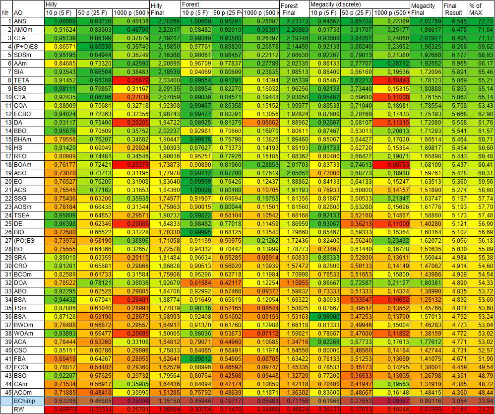
Figure 2. Color-coded ranking of algorithms based on the corresponding tests
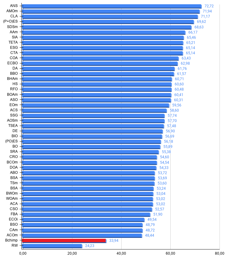
Figure 3. A histogram of the algorithm test results (on a scale from 0 to 100: the higher the score, the better, where 100 is the maximum possible theoretical result); the archive contains a script for calculating the ranking table
Pros and cons of the BChimp algorithm:
Pros:
- Only one external parameter — the population size.
Cons:
- Poor search capabilities.
An archive containing the latest versions of the algorithms' source code is attached to the article. The author of this article is not responsible for the absolute accuracy of the descriptions of canonical algorithms; many of them have been modified to improve search capabilities. The conclusions and judgments presented in the articles are based on the results of the experiments conducted.
Programs used in this article
| # | Name | Type | Description |
|---|---|---|---|
| 1 | #C_AO.mqh | Include file | Parent class for population-based optimization algorithms |
| 2 | #C_AO_enum.mqh | Include file | Enumeration of population-based optimization algorithms |
| 3 | TestFunctions.mqh | Include file | Test function library |
| 4 | TestStandFunctions.mqh | Include file | Test bench function library |
| 5 | TestStand3D.mqh | Include file | 3D visualization panel for the test bench |
| 6 | Utilities.mqh | Include file | Utility function library |
| 7 | CalculationTestResults.mqh | Include file | Script for calculating results for the comparison table |
| 8 | Test_AO_All.mq5 | Script | Unified test bench for all population-based optimization algorithms |
| 9 | Test_AO_AntiCheat | Script | Anti-cheat test for optimization algorithms |
| 10 | Simple use of population optimization algorithms.mq5 | Script | Simple example of using population-based optimization algorithms without visualization |
| 11 | Test_AO_BChimp.mq5 | Script | Test bench for BChimp |
Translated from Russian by MetaQuotes Ltd.
Original article: https://www.mql5.com/ru/articles/23132
Warning: All rights to these materials are reserved by MetaQuotes Ltd. Copying or reprinting of these materials in whole or in part is prohibited.
This article was written by a user of the site and reflects their personal views. MetaQuotes Ltd is not responsible for the accuracy of the information presented, nor for any consequences resulting from the use of the solutions, strategies or recommendations described.