MLP (Multilayer Perceptron) Inside an MQL5 Expert Advisor: Training on Historical Data Without Python or Weight Files
 89
 0

An MLP Trained Inside an Expert Advisor: A Neural Network Without Python or Weight Files
You are developing an MQL5 Expert Advisor and want to add an ML direction filter, but the “train in Python → export weights → load the file” workflow keeps introducing technical risks: normalization mismatches, missing or incorrect versions of weights, and discrepancies in feature logic between the offline environment and the terminal. As a result, the filter may behave erratically, and debugging turns into a search for differences between the two code bases.
The purpose of this article is deliberately practical: not to build a “large neural model,” but to develop a compact MLP gate that is trained on the history of the current symbol and timeframe, is periodically retrained, and operates only on closed bars. While this filter does not replace a full-fledged research ML pipeline, it solves a specific engineering problem for the Expert Advisor: removing external dependencies and making training, features, normalization, and inference part of a single .mq5 file.
Previously, the project’s MLP was trained offline in Python, and a file containing its weights was exported and loaded into the Expert Advisor. This approach worked, but it regularly caused operational problems: different scalers, different feature versions, forgotten files in MQL5\Files, and difficult troubleshooting when behavior in the tester did not match what was expected from the Python model. Here, we propose a different approach: training a small MLP directly within the Expert Advisor itself using historical data from the same instrument on which it will be applied.
The goal of this article is a single, self-contained GridSurvivor_MLP.mq5 file: on a new bar, it assembles a training dataset, generates features and labels without data leakage, trains an MLP with ReLU + softmax, logs validation diagnostics, retrains every N bars, and uses the network’s prediction as the final gate after the divergence check and the HTF filter. The readiness criterion is simple: the network is trained without external files, inference is performed strictly with shift=1, and the behavior when the model is not ready is controlled by InpMlpFailOpen.
Training in the terminal offers three important advantages for a trading robot:
- No normalization mismatches. Features are computed by the same function during both training and inference. The most insidious flaw in the previous approach — the use of different scalers in Python and MQL5 — is eliminated here at the architectural level.
- Adaptation to the instrument and regime. The network learns from actual historical data for a specific symbol and timeframe, rather than from an abstract dataset. When it is launched on GBPUSD, it recognizes the behavior of GBPUSD; when retrained every N bars, it adapts to changes in market regimes.
- Self-sufficiency. The Expert Advisor is distributed as a single file. There are no external dependencies to lose, use the wrong version of, or forget to place in MQL5\Files.
The trade-off is that training in the terminal requires CPU time. Furthermore, a small network using short-term features will not learn what a large model trained on a rich dataset in Python could learn. This is a deliberate trade-off: for an adaptive entry filter, a self-contained design, reproducibility, and ease of maintenance matter more than the highest attainable predictive performance.
What the Network Predicts and How It Is Integrated into the Gate
MLP is not a standalone trading system here. Its role is narrower and more practical: to serve as the final entry filter, answering a single question — whether local market statistics confirm the candidate direction identified by the Expert Advisor's core logic. Therefore, the entire decision-making process looks like this: an RSI divergence identifies a BUY/SELL candidate, the HTF filter checks the higher-timeframe context, and the MLP gate only allows the trade to proceed if there is sufficient alignment between the network’s forecast and the candidate direction.
The network is a two-class classifier: "down" and "up." The input is a feature vector describing the market state on a closed bar; the softmax output consists of two probabilities — P(down) and P(up) — for a horizon of InpMlpHorizon bars ahead. Their difference, P(up) − P(down), represents the network's directional confidence: a positive value indicates an expectation of an increase, while a negative value indicates an expectation of a decrease.
The relationship "label → horizon → gate threshold" is fundamental. The label teaches the network to distinguish which way the price has moved after InpMlpHorizon bars, while InpMlpThreshold sets the minimum margin by which one class must lead the other. If the difference in probabilities is small, the model does not provide a strong enough recommendation, and it is better to reject the candidate.
The RSI divergence continues to generate a candidate with a direction of dir (+1 for BUY, −1 for SELL). The MLP gate accepts a candidate only if the network agrees with that direction with sufficient confidence:
bool ok = (dir == 1) ? (conf >=  InpMlpThreshold)
                   : (conf <= -InpMlpThreshold);
A BUY candidate passes when the network predicts a rise with confidence at or above the threshold; a SELL candidate passes when it predicts a fall. If the divergence points upward but the network confidently predicts a decline, the signal is rejected. This provides dual confirmation: the formal pattern and the learned assessment of direction must agree. The order of the filters remains the same: divergence → HTF filter → MLP. MLP is listed last because it is more expensive than the other checks and should only be triggered for a candidate that has already been found, rather than for every intermediate condition.
Please note: The candidate direction (dir) is not included in the features. The network evaluates the market impartially, predicting its own direction, while alignment with dir is checked externally, in the gate. This is fairer than feeding dir as an input: otherwise, the network could learn simply to repeat the candidate direction.
Features
Each of the eight features can be computed at an arbitrary bar offset shift (this is critical because training iterates over historical bars) and is normalized to a scale on the order of one:
| # | Feature | Formula | Meaning |
|---|---|---|---|
| 0 | RSI Level | rsi[shift] / 50 − 1 | Oversold/Overbought |
| 1 | Short-term RSI slope | (rsi₀ − rsi₃) / 10 | Momentum speed |
| 2 | Long-term RSI slope | (rsi₀ − rsi₆) / 10 | Medium-term dynamics |
| 3 | Distance to EMA(50) | (close − EMA) / ATR | Position Relative to the Trend |
| 4 | Volatility Regime | ATR / (close · 0.001) | Calm or Stormy |
| 5 | Hour (sin) | sin(2π·h / 24) | Trading session, cyclically encoded |
| 6 | Hour (cos) | cos(2π·h / 24) | Trading session, cyclically encoded |
| 7 | Momentum | (close₀ − close₆) / ATR | Magnitude of movement in ATR units |
The distance-to-trend feature uses the EMA(50) of the current timeframe, not a higher timeframe (unlike the HTF entry filter). The reason is technical: the indicator buffer for a higher timeframe is indexed by bars of that timeframe, so accessing it using the current timeframe’s bar shift while iterating through historical data is a recipe for misalignment. The EMA for the current timeframe can be read correctly at any shift using CopyBuffer.
//+------------------------------------------------------------------+
//| Assemble the feature vector at shift (8 values).                 |
//| Computed identically during training and inference → no          |
//| normalization mismatch.                                          |
//+------------------------------------------------------------------+
bool MlpFeatures(int shift, double &f[])
  {
   double rsi[]; ArraySetAsSeries(rsi,true);
   if(CopyBuffer(g_rsiHandle,0,shift,7,rsi)<7) return(false);
   double atr[]; ArraySetAsSeries(atr,true);
   // For ATR, we use the value at shift and the adjacent element to ensure the calculation is correct.
   if(CopyBuffer(g_atrHandle,0,shift,2,atr)<2 || atr[0]<=0.0) return(false);
   double cl[]; ArraySetAsSeries(cl,true);
   if(CopyClose(_Symbol,_Period,shift,7,cl)<7) return(false);
   double ema[]; ArraySetAsSeries(ema,true);
   if(CopyBuffer(g_featMaHandle,0,shift,1,ema)<1) return(false);

   datetime bt = iTime(_Symbol,_Period,shift);
   MqlDateTime mt; TimeToStruct(bt,mt);
   double ang = 2.0*M_PI*mt.hour/24.0;

   ArrayResize(f,MLP_NIN);
   f[0] = rsi[0]/50.0 - 1.0;              // RSI level
   f[1] = (rsi[0]-rsi[3])/10.0;           // short-term RSI slope
   f[2] = (rsi[0]-rsi[6])/10.0;           // long-term RSI slope
   f[3] = (cl[0]-ema[0])/atr[0];          // distance to the EMA in ATR units
   f[4] = atr[0]/(cl[0]*0.001);           // volatility regime
   f[5] = MathSin(ang);                   // hour (cyclic encoding)
   f[6] = MathCos(ang);
   f[7] = (cl[0]-cl[6])/atr[0];           // ATR-normalized momentum
   return(true);
  }
Label
The label for a bar is the direction of future price movement. If the price is higher after InpMlpHorizon bars, the label is class 1 (up); if it is lower, the label is class 0 (down). With series indexing, the future bar is at shift − Horizon (a more recent bar), and when shift > Horizon, it has already closed, so there is no look-ahead bias: at training time, the outcome is known from historical data. The InpLabelMinPts parameter filters out bars with movement below a specified threshold — this acts as a noise filter to prevent the network from learning from price fluctuations around zero.
//+------------------------------------------------------------------+
//| Generating a label for a training example at bar index shift.    |
//| Returns 1 if the price is higher after InpMlpHorizon bars,       |
//| otherwise 0. Filters out noise using InpLabelMinPts.             |
//+------------------------------------------------------------------+
bool MlpLabel(int shift, int &label)
  {
   if(shift < InpMlpHorizon+1) return(false);
   double cn[],cf[];
   if(CopyClose(_Symbol,_Period,shift,1,cn)<1) return(false);
   if(CopyClose(_Symbol,_Period,shift-InpMlpHorizon,1,cf)<1) return(false);
   double move=(cf[0]-cn[0])/_Point;
   if(InpLabelMinPts>0.0 && MathAbs(move)<InpLabelMinPts) return(false);
   label = (move>0.0) ? 1 : 0;
   return(true);
  }
A Network That Learns: The CMlpNet Class
Unlike the inference engine from the previous version, this network is capable of learning. Architecture: input → one hidden layer with ReLU → softmax output for two classes. Weights are stored as flat arrays in row-major order: W1[j·nIn + i] is the weight of the connection from input i to neuron j in the hidden layer, and W2[k·nHid + j] is the weight of the connection from neuron j to output k. He initialization is used with a standard deviation of sqrt(2/n_in), which is appropriate for ReLU.
Forward pass: the hidden layer computes weighted sums and applies ReLU, the output layer produces logits, and softmax converts them into probabilities.
//+------------------------------------------------------------------+
//| Forward pass: input x → class probabilities probs.               |
//| Saves z1 and h for backpropagation.                              |
//+------------------------------------------------------------------+
void Forward(const double &x[], double &probs[])
  {
   for(int j=0;j<m_nHid;j++)
     {
      double z=m_b1[j];
      for(int i=0;i<m_nIn;i++) z+=m_W1[j*m_nIn+i]*x[i];
      m_z1[j]=z; m_h[j]=ReLU(z);
     }
   ArrayResize(probs,m_nOut);
   for(int k=0;k<m_nOut;k++)
     {
      double z=m_b2[k];
      for(int j=0;j<m_nHid;j++) z+=m_W2[k*m_nHid+j]*m_h[j];
      probs[k]=z;
     }
   Softmax(probs,m_nOut);
  }
Training — one SGD step: forward pass, followed by backpropagation of the cross-entropy gradient. For the softmax + cross-entropy pair, the output gradient simplifies to probs[k] − target[k], which is used below. Next, the gradient is passed backward through the hidden layer's ReLU, and the weights are updated according to the rule W ← W − lr · grad.
//+------------------------------------------------------------------+
//| One SGD step: forward pass + backpropagation + weight update.    |
//| Calculates the gradients and updates W1, b1, W2, b2.             |
//+------------------------------------------------------------------+
void Step(const double &x[], int label)
  {
   double probs[]; Forward(x,probs);

   //--- output gradient (softmax + cross-entropy)
   double dOut[]; ArrayResize(dOut,m_nOut);
   for(int k=0;k<m_nOut;k++) dOut[k]=probs[k]-(k==label?1.0:0.0);

   //--- hidden layer gradient (via ReLU)
   double dH[]; ArrayResize(dH,m_nHid);
   for(int j=0;j<m_nHid;j++)
     {
      double g=0.0;
      for(int k=0;k<m_nOut;k++) g+=dOut[k]*m_W2[k*m_nHid+j];
      dH[j]=g*dReLU(m_z1[j]);
     }

   //--- output layer update
   for(int k=0;k<m_nOut;k++)
     {
      for(int j=0;j<m_nHid;j++) m_W2[k*m_nHid+j]-=m_lr*dOut[k]*m_h[j];
      m_b2[k]-=m_lr*dOut[k];
     }
   //--- hidden layer update
   for(int j=0;j<m_nHid;j++)
     {
      for(int i=0;i<m_nIn;i++) m_W1[j*m_nIn+i]-=m_lr*dH[j]*x[i];
      m_b1[j]-=m_lr*dH[j];
     }
  }
A full training cycle runs for a specified number of epochs, shuffling the order of the examples in each epoch using the Fisher–Yates shuffle. Shuffling is important: without it, SGD "drifts" through the examples in chronological order and converges less effectively.
//+------------------------------------------------------------------+
//| Full training cycle on the X/Y dataset.                          |
//| Shuffles examples in each epoch for stable convergence.          |
//+------------------------------------------------------------------+
void Train(const double &X[], const int &Y[], int n, int nIn, int epochs)
  {
   Reset();
   int idx[]; ArrayResize(idx,n);
   for(int i=0;i<n;i++) idx[i]=i;
   for(int ep=0;ep<epochs;ep++)
     {
      //--- Fisher–Yates shuffle
      for(int i=n-1;i>0;i--)
        { int j=MathRand()%(i+1); int t=idx[i]; idx[i]=idx[j]; idx[j]=t; }
      for(int i=0;i<n;i++)
        {
         double xi[]; ArrayResize(xi,nIn);
         int row=idx[i]*nIn;
         for(int f=0;f<nIn;f++) xi[f]=X[row+f];
         Step(xi,Y[idx[i]]);
        }
     }
   m_ready=true;
  }
The correctness of the algorithm has been verified by independently replicating the code. On a synthetic task with a relationship known to be learnable, the network achieves approximately 96% accuracy on the training set. This confirms that the row-major layout of the weights W1[j·nIn+i] / W2[k·nHid+j] is consistent between the forward and backward passes.
Dataset Collection and Training on Historical Data
The TrainModel function builds a training set by iterating through the history from the most recent closed bars to the oldest, calculating the features and label for each bar. Next comes a simple quality assessment: the most recent 20% of bars are set aside for validation, a temporary network is trained on the older 80%, and accuracy is calculated on the held-out bars. This diagnostic result is written to the log and helps determine whether the network provides a useful signal. After evaluation, the final network is trained on the entire sample.
//+----------------------------------------------------------------------+
//| Training dataset collection, validation, and final network training. |
//| Most recent 20% of bars: validation; older 80%: training.            |
//+----------------------------------------------------------------------+
void TrainModel()
  {
   int fromShift = InpMlpHorizon+1;
   int toShift   = MathMin(Bars(_Symbol,_Period)-60, InpMlpHorizon+InpMlpLookback);
   if(toShift <= fromShift+12) return;

   double X[]; int Y[];
   ArrayResize(X, InpMlpLookback*MLP_NIN);
   ArrayResize(Y, InpMlpLookback);
   int cnt=0;
   for(int shift=fromShift; shift<=toShift && cnt<InpMlpLookback; shift++)
     {
      double f[]; int lab;
      if(!MlpFeatures(shift,f)) continue;
      if(!MlpLabel(shift,lab))  continue;
      for(int k=0;k<MLP_NIN;k++) X[cnt*MLP_NIN+k]=f[k];
      Y[cnt]=lab; cnt++;
     }
   if(cnt<80) { Print("GS MLP: insufficient examples: ",cnt); return; }
   ArrayResize(X,cnt*MLP_NIN); ArrayResize(Y,cnt);

   // ... quick validation on the most recent 20% of bars (see the full code) ...

   //--- final network on the entire sample
   if(g_mlp!=NULL) delete g_mlp;
   g_mlp=new CMlpNet(); g_mlp.Init(MLP_NIN,InpMlpHidden,2,InpMlpLR);
   g_mlp.Train(X,Y,cnt,MLP_NIN,InpMlpEpochs);
   g_mlpTrained=true; g_barsSinceTrain=0;
  }
This differs from the Markov indicator. There, the features were constructed from a transition matrix estimated from the data, so when splitting the data into train and validation sets, the matrix had to be built using only the train bars; otherwise, transitions from the validation period would “leak” into the features. In our case, the features are purely local — they are the RSI, ATR, and EMA readings on a single bar and do not depend on any statistics fitted to the dataset. Therefore, there is no data leakage through a shared object, and validation remains unbiased without any additional workarounds. The network still does not see the labels of the validation bars — it is trained only on the training rows.
Integration into the Expert Advisor
The minimum practical integration requires four steps: add the MLP parameters, create an EMA handle for the features, run TrainModel on a new bar, and call MlpAccepts(dir) after the HTF filter in CheckSignal. Everything else consists of network implementation and diagnostic details.
Importantly, the MLP must not directly change the existing trading logic. It only accepts or rejects an already generated candidate. This simplifies debugging: if a candidate appears but no trade is opened, you can separately check the divergence, the HTF filter, network readiness, the conf value, and the InpMlpThreshold threshold in the logs.
A new set of parameters controls both the network and the training:
input group "=== MLP filter (trained in MQL5) ==="
input bool   InpUseMlp       = true;   // Enable the MLP filter
input int    InpMlpHidden    = 24;     // Neurons in the hidden layer
input double InpMlpLR        = 0.01;   // Learning rate
input int    InpMlpEpochs    = 300;    // Training epochs
input int    InpMlpLookback  = 2000;   // Historical bars for training
input int    InpMlpHorizon   = 12;     // Label horizon (bars ahead)
input double InpMlpThreshold = 0.20;   // Confidence threshold |P(up) − P(dn)|
input int    InpRetrainBars  = 250;    // Retrain every N new bars
input double InpLabelMinPts  = 0.0;    // Min. movement for label (0=off)
input bool   InpMlpFailOpen  = false;  // Trade if the network has not been trained
In OnInit, we add initialization of the random number generator for the weights and an EMA handle for the features:
MathSrand((int)TimeCurrent());   // Initialize the generator for the weights
...
g_featMaHandle = iMA(_Symbol, _Period, 50, 0, MODE_EMA, PRICE_CLOSE);
Training is started lazily—on a new bar, rather than in OnInit. The reason is practical: in OnInit, the historical data may not yet be loaded, and CopyBuffer will return only a small amount of data. Data is guaranteed to be available when a new bar arrives. Scheduled retraining is also implemented here:
//--- Train/retrain the network on a new bar
if(InpUseMlp && g_isNewBar)
   if(!g_mlpTrained || (++g_barsSinceTrain >= InpRetrainBars))
      TrainModel();
The gate itself in CheckSignal is a single line after the HTF filter, just as before:
//+--------------------------------------------------------------------------------------------+
//| MLP filter check: Does the network's prediction match dir?                                 |
//| Returns true if the network's confidence exceeds the threshold and its prediction agrees   |
//| with the candidate direction.                                                              |
//+--------------------------------------------------------------------------------------------+
bool MlpAccepts(int dir)
  {
   if(!InpUseMlp) return(true);
   if(!g_mlpTrained || g_mlp==NULL) return(InpMlpFailOpen);
   double f[];
   if(!MlpFeatures(1,f)) return(InpMlpFailOpen);   // the last closed bar
   double pr[]; g_mlp.Forward(f,pr);
   double conf = pr[1]-pr[0];                       // + = up, - = down
   bool ok = (dir==1) ? (conf>= InpMlpThreshold)
                      : (conf<=-InpMlpThreshold);
   return(ok);
  }
Parameters
These parameters form a minimal control panel for the MLP gate. They are used to enable the filter, set the network size, history depth, retraining frequency, label horizon, confidence threshold, and safe behavior when the model is not ready.
| Parameter | Default | Comment |
|---|---|---|
| InpUseMlp | true | Main switch for the MLP filter |
| InpMlpHidden | 24 | 8 features → 16–32 neurons are sufficient; more than that = risk of overfitting |
| InpMlpLR | 0.01 | Higher → faster, but with a risk of divergence; lower → more stable |
| InpMlpEpochs | 300 | Main control over training speed and computational cost |
| InpMlpLookback | 2000 | Smaller → fresher data, but less of it; larger → more stable, but more computationally demanding |
| InpMlpHorizon | 12 | Label horizon; align it with the TP logic/expected grid outcome |
| InpMlpThreshold | 0.20 | Threshold |P(up)-P(down)|; higher → stricter selection, fewer entries |
| InpRetrainBars | 250 | More frequent → more adaptive, but more CPU-intensive |
| InpLabelMinPts | 0.0 | Label noise filter; helps prevent the network from learning from micro-movements |
| InpMlpFailOpen | false | false = do not trade without a trained network; this is safer for live mode |
Pitfalls of Training in the Terminal
The cost of a run in the optimizer. The network is retrained every InpRetrainBars bars, and each training session consists of InpMlpEpochs passes through the dataset. During optimization in the Strategy Tester, this is multiplied by the number of parameter combinations. If the run is slow, increase InpRetrainBars or decrease InpMlpEpochs or InpMlpLookback. For live trading, speed isn't important (one training session every few hundred bars), but for large-scale optimization, it is very important.
Determinism. He initialization uses MathRand. Without controlling the seed, two runs on the same data may yield slightly different weights and different trades. MathSrand fixes the sequence of random numbers within a given run; to reproduce a test exactly, you can replace TimeCurrent() with a constant seed, while for a statistically robust assessment, you should run several sessions with different seeds and examine the variability rather than a single successful run.
Look-ahead bias. This is a common mistake in indicators: the feature on a bar is calculated using future bars. In our Expert Advisor, features are taken strictly from closed bars (inference uses shift=1), while training labels look ahead only within historical data that is already available. At the live edge of the chart, future data does not exist and is not used. It is important to keep this distinction in mind whenever modifying features.
Class imbalance. If the numbers of upward and downward movements for an instrument differ substantially during the training period, the network will be biased toward the more frequent class. The InpLabelMinPts noise filter partially addresses this by filtering out small movements; if there is a significant imbalance, you should add class weighting in Step.
Quick Backtest Check
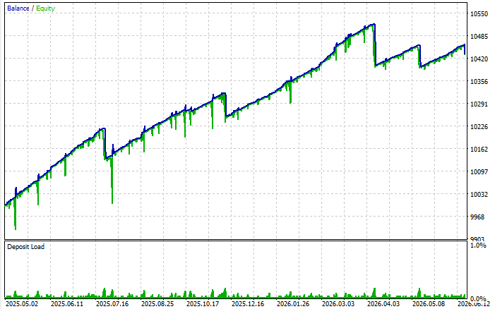
After enabling the MLP gate, evaluate the results not only in terms of profit, but also drawdown behavior, the number of trades, the proportion of rejected candidates, and stability across different historical periods. In one of the tests, the system performs quite well — and the risk manager provides protection by closing problematic series of trades in time:
Here are the detailed statistics:
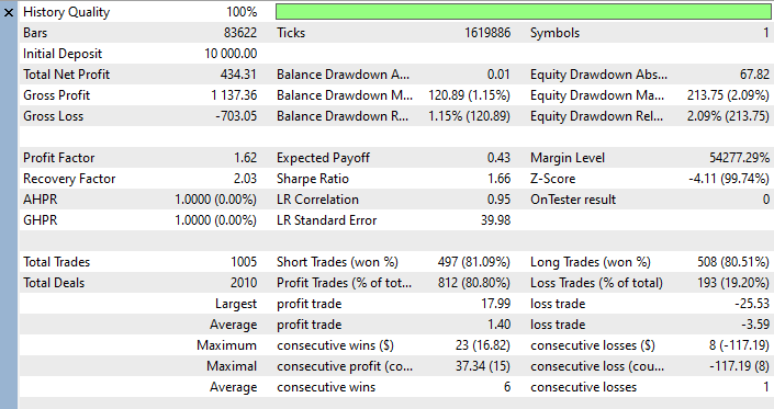
In this backtest, the system achieved a return of 4.34% over one year and one month, with drawdown never exceeding 1.15% and 80% of trades being profitable. This is not proof that the model performs well universally, but an example of an initial check: these results must then be validated across other periods, symbols, spreads, seeds, and retraining parameters.
Checks Before Enabling the MLP gate
Before optimizing the filter or enabling it for live trading, it is helpful to go through a short checklist. It is not just for show, but to ensure that the article actually takes the reader from point A — a chaotic Python/MQL5 pipeline — to point B: a single, testable module within the Expert Advisor.
- The Expert Advisor compiles as a single .mq5 file and does not require an external weights file.
- The logs contain the number of training examples and the accuracy on the held-out historical period.
- Inference in live mode is performed strictly on a closed bar with shift=1.
- Labels are generated based solely on past history and are not included in features.
- The order of the filters in CheckSignal remains the same: divergence → HTF filter → MLP.
- If the network is not ready, its behavior is explicitly controlled by InpMlpFailOpen.
- If there is a significant class imbalance, the label distribution is checked, InpLabelMinPts is adjusted, or class weighting is applied.
- For statistical purposes, multiple runs are performed with different seeds rather than relying on a single impressive result.
Possible Extensions
Normalization layer within the network. Currently, the features are normalized manually using formulas. You can calculate the mean and standard deviation on the training set directly in TrainModel, store them in the network's fields, and apply them in Forward — this way, you can feed features in their natural units, and the network itself will scale them appropriately.
Regression instead of classification. Replace the softmax classifier with a linear output and train it to predict the expected movement in ATR units. The output will then serve not only as a filter but also as a control mechanism: increase InpMaxLevels or the lot size for strong setups.
A second hidden layer or dropout. For a richer feature set, add a second ReLU layer. Using dropout during training reduces overfitting, which is particularly useful when retraining frequently over a short time window.
ONNX for computationally intensive models. If the task outgrows the capabilities of the custom training implementation within the terminal (large networks, convolutions, recurrence), the right approach is to train the model offline and run it using the native OnnxRun function. The custom-built CMlpNet remains ideal for small adaptive networks where zero dependencies and on-the-fly training are valuable.
An ensemble with divergence as a weighted vote. Instead of using a hard gate, combine MLP confidence, HTF agreement, and divergence strength into a single weighted score, then use it to decide both whether to make an entry and how large the position should be.
Outcome
As a result, the MLP has "moved" inside the Expert Advisor: GridSurvivor is now a single, self-contained file that, on new bars, collects features and labels from the historical data for the current symbol/timeframe, validates the dataset, trains the MLP (ReLU + softmax) using SGD steps, and periodically retrains. The network forecast is used as the final filter: divergence suggests a candidate, the HTF filter checks the context, and the MLP confirms the direction based on the rule |P(up)−P(down)| ≥ Threshold; if the model is not ready, behavior is controlled by the InpMlpFailOpen parameter.
The main takeaway isn't that a small network has become "smarter" than a large offline model. The main result is that an entire category of operational errors has been eliminated: mismatched scalers, lost weights, different versions of features, and logic discrepancies between Python and MQL5. Training and inference are now performed using the same code, the same data, and the same feature function.
The completion criterion is simple: the Expert Advisor compiles as a single .mq5 file without external weight files; the logs contain validation metrics; inference is performed strictly at shift=1; and the gate is actually integrated into the decision-making process after divergence and the HTF filter. If the model has not been trained, the Expert Advisor's behavior should not be random — it must be controlled by InpMlpFailOpen.
The limitations remain: training in the terminal is more CPU-intensive, and a small network using short-window features cannot replace sophisticated offline models. For further development, options include built-in normalization, regression instead of classification, an additional hidden layer, dropout, or intensive offline training with deployment via ONNX. However, for an adaptive gate and a reliable operational module, self-containment, transparency, and the absence of external dependencies matter more than the highest achievable model performance.
| File name | File description |
|---|---|
| GridSurvivor_MLP.mq5 | An Expert Advisor with an MLP that trains directly in MQL5 (a single file, no Python, and no weight file) |
Translated from Russian by MetaQuotes Ltd.
Original article: https://www.mql5.com/ru/articles/23172
Warning: All rights to these materials are reserved by MetaQuotes Ltd. Copying or reprinting of these materials in whole or in part is prohibited.
This article was written by a user of the site and reflects their personal views. MetaQuotes Ltd is not responsible for the accuracy of the information presented, nor for any consequences resulting from the use of the solutions, strategies or recommendations described.