

Diebold-Mariano Test in MQL5: Does Your Indicator Actually Forecast Better Than a Random Walk?
 103
 0

Contents
- Introduction
- What the test compares
- Long-run variance and the small-sample correction
- Nested models and the Clark-West adjustment
- The three candidate forecasters
- Scoring forecasts without look-ahead
- Turning the test into a trade gate
- The rolling indicator
- Strategy Tester results
- Limitations
- Conclusion
Introduction
Run two forecasters over a few hundred bars and one will have the lower RMSE. Should an EA trade it? Not until we ask whether the difference is larger than the noise—and decide what kind of evidence should open the gate.
This article builds a rolling forecast filter in plain MQL5. Three models predict the next three-bar return and are compared with a zero-return random walk. Forecasts enter the test only after their outcomes are known. The implementation accounts for overlapping forecast errors, short samples and the different question raised by a nested AR model.
The result is a test library, an Expert Advisor and a chart indicator, with CSV output for independent replay. Together, they help distinguish three claims that require different evidence: lower forecast error, predictive content and trading profit.
What the test compares
Take a forecast made at bar t. The random walk predicts no change, so its error e_RW is just the return that actually happened. Call the model's error e_M. Everything in the test is built on the loss differential:
d_t = L(e_{RW,t}) − L(e_{M,t})
With squared-error loss, a positive d_t means the model beat the random walk on that bar. Under the null, its average is zero and the statistic divides the sample mean by its standard error.
DM = d̄ / √(LRV / T)
This standard error is a common source of mistakes. A three-bar forecast made at bar t and the one made at t+1 share two bars of the same price move, so neighboring values of d_t are correlated. The textbook variance ignores this. Fig. 1 shows the effect in the gold test.
Autocorrelation of the loss differential
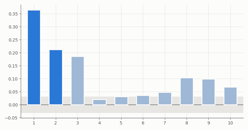
AR model vs. the random walk (XAUUSD H1). The plot uses 3,876 forecasts rebuilt from the per-bar CSV (h = 3), with lags 1 to 10. Dark bars mark the h − 1 lags covered by the rectangular kernel. Light bars are longer lags. The gray band is ±1.96/√T.
Lags one and two, at 0.365 and 0.213, are the overlap. Ignoring them gives −2.95 for this series against −2.00 with them, so the naive number exaggerates the evidence by almost half. But lag three (0.185) and several longer lags are also outside the band. Overlap is not the whole story, and that shapes the variance estimator below.
Long-run variance and the small-sample correction
The long-run variance adds the autocovariances back in. Diebold and Mariano used a rectangular kernel over the first h − 1 lags, which covers the overlap and nothing more. Fig. 1 says that is optimistic for squared returns, so the function has two modes:
//+------------------------------------------------------------------+
//| Long-run variance of a loss-differential series. In guarded mode |
//| the DM rectangular kernel over h-1 lags is used unless it falls  |
//| below DM_RECT_MIN_RATIO of gamma0, in which case (and always in  |
//| Newey-West mode) a Bartlett kernel is used instead.              |
//+------------------------------------------------------------------+
double DMLongRunVariance(const double &x[],const int n,const int h,
                         const ENUM_DM_LRV mode,int &kernel)
  {
   double mean  =DMMean(x,n);
   double gamma0=DMAutocov(x,n,mean,0);
//--- rectangular kernel: covers only the h-1 lags of forecast overlap
   if(mode==DM_LRV_GUARDED)
     {
      double rect=gamma0;
      for(int k=1;k<h;k++)
         rect+=2.0*DMAutocov(x,n,mean,k);
      //--- a near-zero estimate would make the statistic arbitrarily large
      if(rect>0.0 && rect>=DM_RECT_MIN_RATIO*gamma0)
        {
         kernel=DM_KERNEL_RECTANGULAR;
         return(rect);
        }
     }
//--- Bartlett kernel is positive semi-definite by construction
   int    lag =DMNeweyWestLag(n,h);
   double bart=gamma0;
   for(int k=1;k<=lag;k++)
      bart+=2.0*(1.0-k/(lag+1.0))*DMAutocov(x,n,mean,k);
   if(bart>0.0)
     {
      kernel=DM_KERNEL_BARTLETT;
      return(bart);
     }
   kernel=DM_KERNEL_FAILED;
   return(0.0);
  }
In the default guarded mode the rectangular sum is kept only while it stays above 10% of γ_0. The guard exists because of a real case. On XAUUSD M15, the rectangular sum for AR fell to 0.01% of γ_0 during a June stretch. The logged statistic then jumped from −1.02 to −67 in a single bar and peaked at −81. The Bartlett estimate on the same bar gives −0.97. Across all six markets the guard fires on 27 model-bars, every one in that June stretch, and changes no gate decision. InpKernel switches to Newey-West everywhere.
//+------------------------------------------------------------------+
//| Diebold-Mariano test on d = L(benchmark) - L(model). Positive    |
//| statistics favor the model. The HLN factor rescales DM for       |
//| small samples; both one-sided p-values use Student-t(n-1).       |
//+------------------------------------------------------------------+
bool DMTest(const double &d[],const int n,const int h,SDMResult &res,
            const ENUM_DM_LRV mode=DM_LRV_GUARDED)
  {
   DMResetResult(res);
   if(n<DM_MIN_SAMPLE || h<1 || n<=2*h)
      return(false);
   int    kernel=DM_KERNEL_FAILED;
   double lrv   =DMLongRunVariance(d,n,h,mode,kernel);
   if(kernel==DM_KERNEL_FAILED)
      return(false);
//--- raw statistic and the Harvey-Leybourne-Newbold correction
   double mean=DMMean(d,n);
   double dm  =mean/MathSqrt(lrv/n);
   double corr=(n+1.0-2.0*h+h*(h-1.0)/n)/n;
   if(corr<=0.0)
      return(false);
   res.valid  =true;
   res.n      =n;
   res.mean_d =mean;
   res.lrv    =lrv;
   res.kernel =kernel;
   res.dm     =dm;
   res.hln    =dm*MathSqrt(corr);
   res.p_value=1.0-DMStudentTCDF(res.hln,n-1.0);
   res.p_left =DMStudentTCDF(res.hln,n-1.0);
   return(true);
  }
The Harvey, Leybourne and Newbold (1997) factor pulls the statistic in for short samples. Since d_t is benchmark loss minus model loss, p_value is the right tail (model better) and p_left the left tail (random walk better). The gate uses only the right tail.
Nested models and the Clark-West adjustment
Set the AR intercept and every lag coefficient to zero and the forecast is always zero, which is the random walk. So the benchmark lives inside the model. Even when those true values are zero, estimating them from noisy data adds to AR's squared error, and plain DM leans toward "no improvement." Clark and West (2007) add the squared forecast back:
//+------------------------------------------------------------------+
//| Clark-West test for nested models. f is the MSPE-adjusted term:  |
//| e_rw^2 - (e_model^2 - (f_rw - f_model)^2), with f_rw = 0, so it  |
//| is defined for squared loss only. The p-value is the normal      |
//| approximation with no small-sample factor, and for overlapping   |
//| h-step forecasts it relies on the same HAC variance as DM.       |
//+------------------------------------------------------------------+
bool ClarkWestTest(const double &f[],const int n,const int h,
                   SCWResult &res,const ENUM_DM_LRV mode=DM_LRV_GUARDED)
  {
   CWResetResult(res);
   if(n<DM_MIN_SAMPLE || h<1)
      return(false);
   int    kernel=DM_KERNEL_FAILED;
   double lrv   =DMLongRunVariance(f,n,h,mode,kernel);
   if(kernel==DM_KERNEL_FAILED)
      return(false);
   res.valid  =true;
   res.kernel =kernel;
   res.stat   =DMMean(f,n)/MathSqrt(lrv/n);
   res.p_value=1.0-DMNormalCDF(res.stat);
   return(true);
  }
Three caveats apply to the Clark-West adjustment. The term e_RW² − (e_M² − f_M²) is an MSPE comparison, so with absolute loss the EA uses HLN for every model. The p-value is a normal approximation with no small-sample factor. And for overlapping three-bar forecasts I pair it with the same HAC variance as DM, which is common practice but makes the p-value approximate.
The two tests answer different questions. HLN evaluates the model re-estimated over a fixed 300-bar window as it is traded, including estimation noise (the Giacomini-White view). Clark-West tests whether AR contains predictive content, even if the estimated version still loses on MSE. The default gate uses Clark-West for AR and HLN for EMA and LRC. EMA has no fitted parameters. LRC does fit a slope and intercept, but to the last 50 prices, and no restriction on them turns its forecast into zero for every window. Setting the slope to zero still leaves the pull toward the window mean. It is a different model, not a larger one.
The three candidate forecasters
All three predict the next h-bar log return in basis points. EMA extends the latest slope of an EMA of log price. The regression channel projects a 50-bar fitted line h bars ahead and returns its distance from the current price:
//+------------------------------------------------------------------+
//| Regression channel projection: fit a line to the last n log      |
//| prices and return the gap between the line at t+h and the last   |
//| price, in basis points (trend plus pull toward the center)       |
//+------------------------------------------------------------------+
bool DMForecastLRC(const double &lp[],const int count,const int n,
                   const int h,double &forecast)
  {
   forecast=0.0;
   if(n<3 || count<n)
      return(false);
   int    start=count-n;
   double x_bar=(n-1)/2.0;
   double y_bar=0.0;
   for(int i=0;i<n;i++)
      y_bar+=lp[start+i];
   y_bar/=n;
//--- ordinary least squares slope and intercept
   double sxy=0.0;
   double sxx=0.0;
   for(int i=0;i<n;i++)
     {
      double dx=i-x_bar;
      sxy+=dx*(lp[start+i]-y_bar);
      sxx+=dx*dx;
     }
   if(sxx<=0.0)
      return(false);
   double slope    =sxy/sxx;
   double intercept=y_bar-slope*x_bar;
   double projected=intercept+slope*(n-1+h);
   forecast=(projected-lp[count-1])*DM_SCALE;
   return(true);
  }
AR fits an intercept and p lags by OLS on the last 300 one-bar returns, then rolls the equation forward h steps:
//+------------------------------------------------------------------+
//| h-bar AR(p) forecast: iterate the fitted recursion h steps and   |
//| add up the predicted one-bar returns                             |
//+------------------------------------------------------------------+
bool DMForecastAR(const double &lp[],const int count,const int p,
                  const int m,const int h,double &forecast)
  {
   forecast=0.0;
   double coef[];
   if(!DMFitAR(lp,count,p,m,coef))
      return(false);
//--- hist[0] is the newest known return, hist[p-1] the oldest
   double hist[];
   ArrayResize(hist,p);
   for(int lag=0;lag<p;lag++)
      hist[lag]=(lp[count-1-lag]-lp[count-2-lag])*DM_SCALE;
   double total=0.0;
   for(int step=0;step<h;step++)
     {
      double next=coef[0];
      for(int lag=1;lag<=p;lag++)
         next+=coef[lag]*hist[lag-1];
      total+=next;
      for(int lag=p-1;lag>0;lag--)
         hist[lag]=hist[lag-1];
      hist[0]=next;
     }
   forecast=total;
   return(true);
  }
Both functions take their lengths as arguments. The values used in every test (n = 50 for LRC, p = 3 lags and m = 300 bars for AR, the 250-bar rolling window and the gate statistic) are the EA's default inputs:
//+------------------------------------------------------------------+
//| Input parameters                                                 |
//+------------------------------------------------------------------+
input group "Forecast evaluation"
input ENUM_TIMEFRAMES InpTimeframe    = PERIOD_CURRENT;          // Timeframe the EA samples
input int             InpHorizon      = 3;                       // Forecast horizon h (bars)
input int             InpWindow       = 250;                     // Rolling DM window W
input ENUM_DM_LOSS    InpLoss         = DM_LOSS_SQUARED;         // Loss function
input ENUM_DM_SELECT  InpModelSelect  = SELECT_AUTO;             // Model(s) to trade
input bool            InpGateEnabled  = true;                    // Require significant DM edge
input ENUM_GATE_TEST  InpGateTest     = GATE_TEST_NESTED_AWARE;  // Gate statistic
input ENUM_DM_LRV     InpKernel       = DM_LRV_GUARDED;          // Long-run variance estimator
input double          InpAlpha        = 0.05;                    // One-sided significance level
input bool            InpBonferroni   = true;                    // Divide alpha by models tested
input group "Candidate models"
input int             InpEMAPeriod    = 20;                      // EMA period
input int             InpLRCPeriod    = 50;                      // Regression channel length
input int             InpAROrder      = 3;                       // AR order p
input int             InpARWindow     = 300;                     // AR estimation window
input double          InpMinForecast  = 0.0;                     // Min |forecast| to trade (bps)
input group "Risk and execution"
input double          InpRiskPercent  = 0.5;                     // Risk per trade (% equity)
input int             InpATRPeriod    = 14;                      // ATR period
input double          InpStopATR      = 1.5;                     // Stop loss (x ATR)
input double          InpTargetATR    = 2.0;                     // Take profit (x ATR)
input int             InpHoldBars     = 0;                       // Time exit in bars (0 = h)
input ulong           InpMagic        = 26092301;                // Magic number
input group "Logging and checks"
input bool            InpLogCSV       = true;                    // Per-bar CSV in Common Files
input string          InpLogFolder    = "DieboldMariano";        // Common Files subfolder
input bool            InpRunSelfTest  = true;                    // Run numeric self-test at start
These values were fixed before the tests and were not tuned. The horizon h = 3 is short enough to trade but long enough for forecast overlap to matter. A 250-bar window covers about ten trading days on H1 and under three on M15. The AR window is longer than the rolling window, and the EMA and LRC lengths are common chart settings. I did not test other values, so the results below apply only to these parameters.
Scoring forecasts without look-ahead
It is easy to leak the future by scoring a forecast before its three bars have closed. CRollingDM holds h open forecasts in a ring and, on each bar, scores the one made exactly h bars ago before storing the new one.
//+------------------------------------------------------------------+
//| Close the origin opened h bars ago, then open a new one.         |
//| Returns true when a realized error pair entered the window.      |
//+------------------------------------------------------------------+
bool CRollingDM::Update(const double log_price,const double forecast,
                        const bool forecast_ok,const bool record)
  {
   int  slot =(int)(m_tick%m_h);
   bool added=false;
   if(m_pend_ok[slot])
     {
      //--- realized h-bar return versus both forecasts
      double fc    =m_pend_fc[slot];
      double y     =(log_price-m_pend_lp[slot])*DM_SCALE;
      double e_mod =y-fc;                                        // model error
      double e_rw  =y;                                           // random walk predicts zero
      double d     =DMLoss(e_rw,m_loss)-DMLoss(e_mod,m_loss);    // > 0 favors the model
      double f     =e_rw*e_rw-(e_mod*e_mod-fc*fc);               // Clark-West term, squared loss
      m_win_d[m_head] =d;
      m_win_f[m_head] =f;
      m_win_lm[m_head]=DMLoss(e_mod,m_loss);
      m_win_lr[m_head]=DMLoss(e_rw,m_loss);
      m_head=(m_head+1)%m_window;
      if(m_filled<m_window)
         m_filled++;
      //--- full-sample store, used for the end-of-test verdict
      if(record)
        {
         ArrayResize(m_all_d,m_all_n+1,4096);
         ArrayResize(m_all_f,m_all_n+1,4096);
         m_all_d[m_all_n]=d;
         m_all_f[m_all_n]=f;
         m_all_n++;
         m_sse_model+=e_mod*e_mod;
         m_sse_rw   +=e_rw*e_rw;
        }
      added=true;
     }
   m_pend_lp[slot]=log_price;
   m_pend_fc[slot]=forecast;
   m_pend_ok[slot]=forecast_ok;
   m_tick++;
   return(added);
  }
Warm-up bars pass record as false, so they fill the rolling window but stay out of the full-sample verdict. That sets the sample sizes. The EA scores every forecast realized inside the test, which includes three issued during warm-up (3,879 on XAUUSD H1). The per-bar CSV starts at the first test bar, so series rebuilt from it, including Fig. 1 and the replays below, have three fewer (3,876). Those replays match the EA's logged rolling statistics to 1e-4, apart from the near-zero-variance bars above, and its gate decisions on every bar.
Turning the test into a trade gate
Once per bar the EA updates the evaluators, runs the tests and asks SelectModel() whether any model has earned a trade:
//+------------------------------------------------------------------+
//| Pick the model to trade on this bar; -1 means stay flat          |
//+------------------------------------------------------------------+
int SelectModel(SDMResult &dm[],SCWResult &cw[],double &alpha_eff)
  {
   int candidates=0;
   for(int m=0;m<DM_MODEL_COUNT;m++)
      if(ModelAllowed(m))
         candidates++;
   alpha_eff=InpAlpha;
   if(InpBonferroni && candidates>1)
      alpha_eff=InpAlpha/candidates;
   int    best      =-1;
   double best_score=DBL_MAX;
   for(int m=0;m<DM_MODEL_COUNT;m++)
     {
      if(!ModelAllowed(m) || !g_forecast_ok[m])
         continue;
      if(InpGateEnabled)
        {
         //--- gated: only the statistic that decides must be valid
         bool   use_cw=UsesClarkWest(m);
         bool   valid =use_cw ? cw[m].valid : dm[m].valid;
         double p     =use_cw ? cw[m].p_value : dm[m].p_value;
         if(!valid)
            continue;
         //--- right tail only: the model must beat the random walk
         if(p<alpha_eff && p<best_score)
           {
            best_score=p;
            best      =m;
           }
        }
      else
        {
         //--- ungated control: lowest rolling loss wins, no test
         if(!dm[m].valid)
            continue;
         double loss=g_dm[m].WindowLossModel();
         if(loss<best_score)
           {
            best_score=loss;
            best      =m;
           }
        }
     }
   return(best);
  }
Only the statistic that makes the decision has to be valid, and only the right tail counts. With three models at 5% each, the chance that one passes by luck would be about 14% if the tests were independent. They are correlated, so it is lower, and the Bonferroni cut to 0.0167 caps it at 5% either way. With InpGateEnabled off, the function becomes the control and takes the model with the lowest recent error.
What an open gate means depends on the model. For EMA and LRC the gate uses HLN, so it opens only when the rolling squared error is significantly lower than the random walk's. For AR the default gate uses Clark-West, so an open AR gate is evidence of predictive content, not proof that the estimated AR has the lower rolling error. Its HLN statistic can still be negative on the same bar. The selection rule is in UsesClarkWest():
//+------------------------------------------------------------------+
//| True when the gate for this model uses Clark-West                |
//+------------------------------------------------------------------+
bool UsesClarkWest(const int model)
  {
//--- the Clark-West term is an MSPE comparison, so it needs squared loss
   if(InpLoss!=DM_LOSS_SQUARED)
      return(false);
   if(InpGateTest==GATE_TEST_CLARK_WEST)
      return(true);
   if(InpGateTest==GATE_TEST_HLN)
      return(false);
   return(model==DM_MODEL_AR);
  }
To trade every model, AR included, only on significantly lower error, set InpGateTest to GATE_TEST_HLN. The replay below reports this variant as "HLN for AR too".
The forecast sign decides direction, stops and targets are ATR multiples, and positions close after h bars. Lot size is cross-checked against contract size. That check fired in every gold run because this server reports XAUUSD tick value ten times too small.
The rolling indicator
The indicator runs the same engine and evaluator on closed chart bars and draws one line, the right-tail threshold, since the lower tail plays no part in the gate:
//+------------------------------------------------------------------+
//| Custom indicator iteration function                              |
//+------------------------------------------------------------------+
int OnCalculate(const int rates_total,
                const int prev_calculated,
                const int begin,
                const double &price[])
  {
//--- full recalculation on first call or when history changes
   if(prev_calculated==0 || prev_calculated>rates_total)
     {
      g_engine.Reset();
      g_dm.Reset();
      ArrayInitialize(g_hln,EMPTY_VALUE);
      ArrayInitialize(g_cw,EMPTY_VALUE);
      ArrayInitialize(g_gate,EMPTY_VALUE);
      g_next=begin;
      if(InpMaxBars>0)
         g_next=MathMax(begin,rates_total-InpMaxBars);
     }
//--- only closed bars enter the test; the forming bar stays empty
   int last_closed=rates_total-2;
   for(int i=g_next;i<=last_closed;i++)
     {
      g_hln[i] =EMPTY_VALUE;
      g_cw[i]  =EMPTY_VALUE;
      g_gate[i]=EMPTY_VALUE;
      if(price[i]<=0.0)
         continue;
      double lp=MathLog(price[i]);
      double fc=0.0;
      g_engine.Push(lp);
      bool ok=g_engine.Forecast(InpModel,InpHorizon,fc);
      g_dm.Update(lp,fc,ok,false);
      SDMResult dm;
      SCWResult cw;
      if(!g_dm.Evaluate(dm,cw))
         continue;
      g_hln[i] =dm.hln;
      g_cw[i]  =cw.valid ? cw.stat : EMPTY_VALUE;
      //--- only the right tail matters: the model must beat the benchmark
      g_gate[i]=g_crit;
     }
   if(last_closed+1>g_next)
      g_next=last_closed+1;
//--- forming bar
   if(rates_total>0)
     {
      g_hln[rates_total-1] =EMPTY_VALUE;
      g_cw[rates_total-1]  =EMPTY_VALUE;
      g_gate[rates_total-1]=EMPTY_VALUE;
     }
   return(rates_total);
  }
Rolling HLN and Clark-West statistics for AR, XAUUSD H1
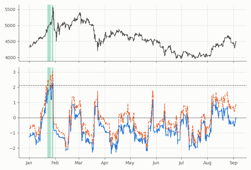
Top: close price. Bottom: HLN (solid blue) and Clark-West (dashed orange) over a 250-bar window, as logged by the EA. The dotted line is the right-tail gate threshold for Clark-West, 2.13 (one-sided, α = 0.05/3). Green shading marks bars where the gate was open.
The orange line spends most of the year above the blue one. Part of that is mechanical, because the Clark-West term adds f_M² ≥ 0 to every d_t. How big the gap gets also depends on forecast size, the variance estimate and the window, so it should not be read as a measure of nesting bias alone. In late January Clark-West crossed the line and the gate was open for 90 bars. HLN crossed its 2.14 threshold on 11 bars in the whole test.
Strategy Tester results
Every test used MetaQuotes-Demo, real ticks, a $10,000 deposit, 1:100 leverage, a 5 ms delay and default inputs. H1 covers 2026.01.02 to 2026.09.04 and M15 2026.06.01 to 2026.09.04. Each market ran once with the gate on and once with it off. Both runs score the same forecasts, so they share one full-sample verdict. RMSE is in basis points of the three-bar return.
The balances also depend on the account and symbol settings:
| Setting | Value |
|---|---|
| Server and account | MetaQuotes-Demo, hedging account in USD |
| Deposit and leverage | $10,000, 1:100 |
| Modeling and delay | Every tick based on real ticks, 5 ms |
| Spread | Bid and ask of the recorded real ticks |
| Commission | None charged in these runs |
| Swaps | Charged by the tester from the symbol specification, not logged per deal |
| Contract size | 100,000 for EURUSD and GBPUSD, 100 oz for XAUUSD |
| Minimum volume | 0.01 lot |
| EA inputs | Defaults shown above, with InpGateEnabled true or false |
Three of these need a note. No commission appeared: balances rebuilt from deal prices alone match the tester to the cent in runs with no position held overnight. Swaps did apply: the ungated runs, with 59 to 172 overnight positions, end $23 to $48 below their rebuilt balances. On XAUUSD the server reports a tick value ten times too small, so the EA sized gold positions from the 100-oz contract size instead. Rebuilding the gated XAUUSD H1 run at 100 oz gives $10,272.01 against the tester's $10,271.62. EURUSD and GBPUSD needed no adjustment.
| Market | n | RMSE RW | RMSE EMA | RMSE LRC | RMSE AR | HLN EMA | HLN LRC | HLN AR | CW AR |
|---|---|---|---|---|---|---|---|---|---|
| XAUUSD H1 | 3,879 | 69.85 | 74.46 | 134.55 | 70.84 | −3.23 | −9.99 | −2.00 | −0.86 |
| EURUSD H1 | 4,198 | 13.07 | 14.05 | 23.28 | 13.23 | −6.25 | −13.45 | −3.53 | −1.33 |
| GBPUSD H1 | 4,196 | 14.55 | 15.63 | 26.72 | 14.72 | −6.65 | −14.44 | −3.32 | −1.28 |
| XAUUSD M15 | 6,050 | 27.44 | 29.34 | 50.10 | 27.75 | −6.42 | −15.04 | −3.14 | 0.33 |
| EURUSD M15 | 6,624 | 5.51 | 5.88 | 10.84 | 5.57 | −5.18 | −13.44 | −2.21 | 0.85 |
| GBPUSD M15 | 6,624 | 6.10 | 6.53 | 11.43 | 6.19 | −5.88 | −13.28 | −3.78 | −0.90 |
Full-sample HLN statistics by model and market
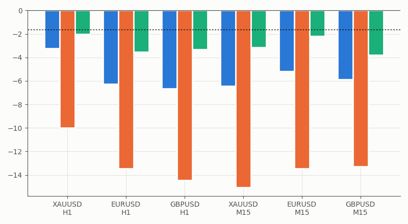
Bars in each group: EMA (blue), regression channel (orange), AR (green). The dotted line is the left-tail 5% level, −1.645. A bar below it means the random walk was significantly more accurate.
Every model has a higher RMSE than the random walk in every market. That conclusion needs the left tail, so I read it from p_left. All eighteen are below 0.05, and sixteen stay significant after dividing 5% by eighteen. The two that don't are AR on XAUUSD H1 (p = 0.023) and EURUSD M15 (0.014). The regression channel's RMSE is 1.8 to 2.0 times the random walk's in every market. Its pull toward the channel center bets on a reversion that three-bar returns do not deliver. Rebuilt using Newey-West on the CSV series, all eighteen still fall below −1.645, the weakest being AR on XAUUSD H1 at −1.89. The kernel does not change this verdict.
The gate is a separate question, decided bar by bar on 250-bar windows. The replay counts open bars under each variant:
| Market | Bars | As run | Newey-West | CW with HLN factor | HLN for AR too |
|---|---|---|---|---|---|
| XAUUSD H1 | 3,627 | 90 | 122 | 86 | 11 |
| EURUSD H1 | 3,946 | 0 | 0 | 0 | 0 |
| GBPUSD H1 | 3,944 | 10 | 13 | 5 | 0 |
| XAUUSD M15 | 5,798 | 22 | 33 | 19 | 0 |
| EURUSD M15 | 6,372 | 94 | 100 | 87 | 18 |
| GBPUSD M15 | 6,372 | 109 | 147 | 106 | 0 |
A small-sample factor on Clark-West trims openings from 325 to 303, while Newey-West raises them to 415. The largest effect comes from the test chosen for AR. Judge the estimated AR with HLN and the gate opens on 29 bars instead of 325.
| Market | Gate open | Trades ON | Balance ON | Trades OFF | Balance OFF |
|---|---|---|---|---|---|
| XAUUSD H1 | 2.32% | 26 | $10,271.62 | 1,271 | $9,582.87 |
| EURUSD H1 | 0.00% | 0 | $10,000.00 | 1,572 | $7,536.17 |
| GBPUSD H1 | 0.24% | 4 | $9,934.56 | 1,573 | $5,974.25 |
| XAUUSD M15 | 0.36% | 9 | $10,009.43 | 2,201 | $6,284.36 |
| EURUSD M15 | 1.42% | 34 | $10,049.70 | 2,419 | $6,168.91 |
| GBPUSD M15 | 1.65% | 41 | $9,899.70 | 2,417 | $4,895.71 |
GBPUSD H1 balance, gate ON and OFF
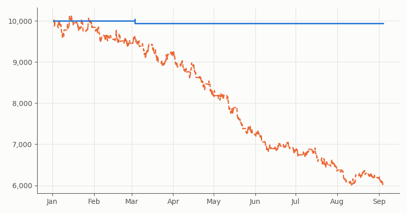
Gate ON solid blue, gate OFF dashed orange, rebuilt deal by deal from the tester journal as price change × volume × 100,000. The journal omits swaps. The ON curve, with no overnight position, matches the tester to the cent. The OFF curve, with 172 overnight positions, ends at $6,012.09 against the tester's $5,974.25.
Net return by market, gate ON and OFF
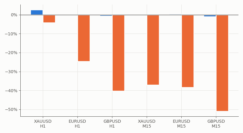
Gate ON blue, gate OFF orange, from the Strategy Tester's final balances.
The ungated runs lost 4.2% to 51.0%. That gap mostly measures exposure, not the test: the gated EA took 0 to 41 trades per run against 1,271 to 2,419, and paid the spread far less often. Trading P/L also depends on stops, targets, position sizing and the exit rule. The test does not model these components. To separate the filter from the exposure, I split the ungated trades by whether the gate was open on their decision bar. The 108 taken on open bars averaged +$2.82 with a 53.7% win rate. The 11,345 taken on closed bars averaged −$1.73 with 47.0%. The difference points the right way, but at p = 0.07 (Welch) it is not significant. P/L here is price change × volume × contract size, without swaps.
The gate's open rate, 0% to 2.3%, is close to the 1.7% a 0.0167 threshold would give by chance. That is only a rough benchmark, because overlapping windows make the tests dependent and the p-values need not be exactly uniform.
Limitations
Short windows and dependence. Bonferroni covers the three models on one bar, not thousands of overlapping windows, so some openings will be false alarms.
Self-test scope. The 30 checks cover the distributions, h = 1, 2 and 3, the Bartlett fallback, Clark-West and the forecasters. They do not cover absolute loss or other horizons. I checked the guard separately by running the translated code on 5,495 real XAUUSD M15 bars against an independent Python replay, with a largest difference of 1e-10.
Minimum lot. In the gated XAUUSD H1 run, 19 signals were skipped because 0.5% risk bought less than 0.01 lot at late-January ATR levels.
Fixed parameters. The horizon, the rolling window, the AR window and order, and the EMA and LRC lengths were set once and never varied. The full-sample verdicts, gate frequencies and balances hold only for these settings, and neighboring values may give different results.
One period, three markets. These results cover 2026 data on one demo server.
Conclusion
This article follows forecasts from their realized errors to rolling test statistics and trade decisions. The MQL5 tools provide a practical workflow: score forecasts only after their horizon closes, use the HLN test to assess realized accuracy, and use Clark–West when asking whether the nested AR model contains predictive content. The indicator displays the rolling evidence; the EA applies the selected threshold and logs its decisions for inspection.
In these tests, with the default parameters, none of the three models achieved a lower full-sample RMSE than the random walk. The benchmark was significantly more accurate in 16 of 18 comparisons after applying a Bonferroni correction for those 18 comparisons. The trading gate sharply reduced exposure, but the results do not establish that its selected trades are profitable. Bonferroni controls the three model tests on each bar; it does not remove the risk of false openings from repeated, overlapping rolling tests. Nor does the guarded variance estimate necessarily capture dependence beyond the forecast-overlap lags.
Use the tools to audit a forecast before treating it as a trading signal: choose the test that matches the claim, inspect the rolling statistic and threshold, and replay the logged decisions. A passing test is evidence about a forecast—not a certificate of trading profitability.
| File | Type | Description |
|---|---|---|
| MQL5\Include\DieboldMariano\DieboldMarianoCore.mqh | Include | DM, HLN and Clark-West tests, guarded and Newey-West variance, distributions, forecasters, CForecastEngine, CRollingDM and the self-test. |
| MQL5\Experts\DieboldMariano\DMForecastGate_EA.mq5 | Expert Advisor | Trades a model only while its gate test passes (HLN for EMA and LRC, Clark-West for AR by default); logs per-bar and summary CSVs to Common Files. |
| MQL5\Indicators\DieboldMariano\DMRollingStat.mq5 | Indicator | Plots the rolling HLN and Clark-West statistics with the right-tail threshold. |
| MQL5\Files\DieboldMariano\*.py | Python | Reference implementation, self-test values and the offline gate replay. |
Warning: All rights to these materials are reserved by MetaQuotes Ltd. Copying or reprinting of these materials in whole or in part is prohibited.
This article was written by a user of the site and reflects their personal views. MetaQuotes Ltd is not responsible for the accuracy of the information presented, nor for any consequences resulting from the use of the solutions, strategies or recommendations described.


