Survival Analysis for Trade Exits: A Discrete-Time Competing-Risks Model in MQL5

Introduction

Most of the effort in a trading system goes into the entry. We optimise the filter, tune the lookback, argue about confirmation. Then we bolt on a two-to-one take-profit and a one-ATR stop and stop thinking about it. That fixed exit throws away everything the market tells us after we are in the trade.

Think about what happens once a position is open. It runs one and a half R in your favour and stalls. Volatility doubles. Price falls back through the moving average it broke out from. Each of those facts changes the probability of hitting the target before the stop. A fixed exit ignores them.

Medical statistics solved a version of this decades ago. A live position is a patient under observation. Each bar it survives is one more period at risk, leaving the study one of two mutually exclusive ways: take-profit fires, or stop-loss fires. Those are competing risks — one happening permanently prevents the other. If the time stop arrives first, the observation is censored.

That framing fixes two things a naive "will this trade win?" classifier gets wrong. A trade still open at the time stop is a censored observation, not a failed prediction. And trade state is not static — MFE, MAE, distance to each barrier and the volatility regime all move while the position lives. A discrete-time hazard model eats time-varying covariates naturally; a classifier scored once at entry cannot.

What follows is a complete native MQL5 implementation. It uses no DLLs, no ONNX runtime, and no ALGLIB. We harvest a person-period table and fit two cause-specific hazards by penalised maximum likelihood. We then convert cumulative incidence into a bar-by-bar hold-or-close decision. The result is tested against fixed exits on four instruments with every parameter identical, and reported including the parts that performed poorly.

Contents

1. Why an exit is a survival problem
2. Cause-specific hazards and cumulative incidence
3. Building the person-period table
4. Fitting the model natively in MQL5
5. From cumulative incidence to an exit decision
6. Edge cases and pitfalls
7. Testing in the Strategy Tester
8. Conclusion

Why an exit is a survival problem

Start with the quantity you actually want. At bar t of an open position: given it is still alive and given what the chart looks like now, what is the probability it reaches target before stop? Not "is this a good trade" — that was settled at entry. The question is conditional on survival.

That conditional-on-survival structure is what a hazard function encodes. The discrete-time hazard for cause j is the probability the trade exits via cause j during bar t, given it was open at the start of bar t:

h j (t | x t ) = P( T = t, J = j | T ≥ t, x t )

where T is the bar index of the exit, J is the cause (1 = take-profit, 2 = stop-loss), and x t is the state of the trade and the market measured at the start of bar t.

Two features make this a good fit for trading. The conditioning set is the at-risk population, so trades that have already exited drop out. And the covariate vector carries a subscript t: it may change every bar.

Why this is a competing-risks problem rather than two independent survival problems is easy to get wrong. Censoring means "we stopped watching" — the event could still have happened. When a stop fires, the take-profit becomes impossible, not unobserved. Treating one barrier as censoring for the other describes a world where stops do not exist, and the numbers come out too optimistic.

Scope. This article models exits only. The entry rule's code and parameters — a 20-bar Donchian breakout gated on elevated ATR — are held byte-identical across instruments and both arms. That is a test-design choice, not a recommendation: as the results show, it is a fairly weak filter on its own. It exists here to isolate the exit policy, the only thing this article claims anything about.

Cause-specific hazards and cumulative incidence

Because exactly one of three things happens on each bar at risk — take-profit, stop-loss, or survive — the two cause-specific hazards fall straight out of a multinomial logit with "survive" as the reference category:

ηj(t) = βj' z(t, xt)

hj(t) = exp(ηj) / ( 1 + exp(η1) + exp(η2) )

The design row is z(t, x t ) = [ 1, log t, t/T max , x 1 … x p ]. The two time terms are the baseline hazard. Survival through bar t is the product of per-bar survival, and cumulative incidence for cause j accumulates hazard weighted by the probability of having got that far:

S(t) = ∏s=1..t [ 1 − h1(s) − h2(s) ]

Fj(t) = ∑s=1..t hj(s) · S(s−1)

Note that F j (t) is not 1 − S(t). The S(s−1) factor is the point: a large hazard at bar 60 contributes almost nothing if three percent of trades are still alive by then. F 1 + F 2 + S(T max ) sums to 1. This is verified on the fitted XAUUSD model and holds to 12 decimal places.

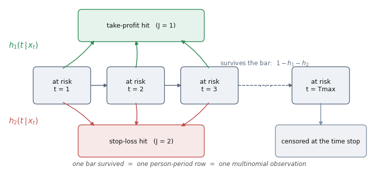
Fig. 1. The state structure. A position moves along the at-risk chain one bar at a time, and on each bar it is absorbed into one of two exit states or survives to the next. A trade still at risk at the time stop is censored, not lost, and each bar survived becomes one row of the estimation table.

Building the person-period table

The structure that makes this work is the person-period table: one row per trade per bar at risk. A trade hitting its stop after nine bars contributes nine rows — eight "survived", one "stop-loss". No special term for censoring: the censored trade simply stops generating rows.

The covariates are nine time-varying measurements, all scale-free so the coefficients mean something across volatility regimes:

Covariate	Definition	What it is meant to capture
mfe_R	max favourable excursion/risk	how much the trade has already given you
mae_R	max adverse excursion/risk	how much heat it has taken
cur_R	unrealised result in R	where it stands right now
dist_tp_atr	(target − price)/ATR(14)	ATRs of travel still required
dist_sl_atr	(price − stop)/ATR(14)	room before the stop is reached
vol_ratio	ATR(14)/ATR(50)	volatility expansion since entry
range_pos	signed position in the 20-bar range	whether the breakout is extending
trend_align	(price − EMA50)/ATR(14), signed	agreement with the medium trend
park_ratio	Parkinson 20-bar vol/ATR(14)	realised range against typical range

Everything signed is multiplied by trade direction, so a short position's covariates read the same way a long's do.

The most valuable piece of defensive engineering here is the feature contract. The builder returns the number of covariates it actually wrote, and every component compares that with the compiled constant before it is allowed to touch the market:

//--- Returns the number of covariates actually written. The caller
//--- compares that with SURV_NUM_FEATURES - this is the contract test.
int CSurvivalFeatures::Build(const STradeState &st, const SMarketSnapshot &mk, double &x[])
  {
   ArrayResize(x, SURV_NUM_FEATURES);
   if(st.risk <= 0.0 || mk.atr14 <= 0.0)
      return(0);

   double cur_R = st.dir * (mk.close - st.entry) / st.risk;
   double rng   = MathMax(mk.hi20 - mk.lo20, _Point);
   int n = 0;
   x[n++] = st.mfe_R;
   x[n++] = st.mae_R;
   x[n++] = cur_R;
   x[n++] = st.dir * (st.tp - mk.close) / mk.atr14;
   x[n++] = st.dir * (mk.close - st.sl) / mk.atr14;
   x[n++] = mk.atr14 / mk.atr50;
   x[n++] = st.dir * (2.0 * (mk.close - mk.lo20) / rng - 1.0);
   x[n++] = st.dir * (mk.close - mk.ema50) / mk.atr14;
   x[n++] = mk.park20 / mk.atr14;

   for(int k = 0; k < n; k++)
      x[k] = MathMax(-SURV_CLIP, MathMin(SURV_CLIP, x[k]));
   return(n);
  }

The check runs three ways: the compiled constant, the builder's return value, and the manifest width. If the constant is not updated, the EA refuses to initialise and reports the mismatch. This prevents reading trend_align into the coefficient trained for vol_ratio.

Both the harvester and the live EA read covariates through one shared object, CSeriesCache — a correctness decision, not a performance one. Separate code paths for training and live features often cause deployed models to break silently.

Row ordering is where leakage creeps in. Covariates for period t come from the bar that closed before period t begins; the outcome comes from the bar period t plays out in:

for(int t = 1; t <= m_tmax; t++)
  {
   int idx_obs = i - (t - 1);  // bar that closed before period t
   int idx_evt = i - t;        // bar in which period t plays out

   SMarketSnapshot mk;
   c.Snapshot(idx_obs, mk);
   st.bars_held = t - 1;
   CSurvivalFeatures::Build(st, mk, xs);

   //--- Resolve period t on the event bar.
   double hi = c.High(idx_evt), lo = c.Low(idx_evt);
   bool hit_tp = (dir > 0 ? hi >= st.tp : lo <= st.tp);
   bool hit_sl = (dir > 0 ? lo <= st.sl : hi >= st.sl);

   int y = SURV_EV_SURVIVE;
   if(hit_sl)
      y = SURV_EV_SL;
   else if(hit_tp)
      y = SURV_EV_TP;

On a real run across four instruments, M30, 2023.01.01–2025.06.30, this produced between 6,422 and 7,923 person-period rows per instrument from 997 to 1,055 virtual trades. Only one virtual trade runs at a time, so overlapping trades never inflate the effective sample.

Fitting the model natively in MQL5

Stack the coefficient blocks into θ = [β 1 ; β 2 ]. With nine covariates the design dimension is twelve, so θ has 24 elements and the information matrix is 24 × 24 — which the native matrix type inverts in microseconds:

gj = ∑i zi ( yij − pij ) − λ βj

A(j,k) = ∑i zi zi' ( pij δjk − pij pik ) + λ I

θ ← θ + A−1 g

The 2 × 2 weight block per row is the multinomial variance: p1(1-p1) and p2(1-p2) on the diagonal, -p1*p2 off it. The off-diagonal is negative because the causes compete for the same probability mass.

double r1 = y1 - p1;
double r2 = y2 - p2;
double w11 = p1 * (1.0 - p1);
double w22 = p2 * (1.0 - p2);
double w12 = -p1 * p2;

for(int a = 0; a < d; a++)
  {
   g[a]     += z[a] * r1;
   g[d + a] += z[a] * r2;
  }

for(int a = 0; a < d; a++)
  {
   double za = z[a];
   if(za == 0.0)
      continue;
   for(int b = a; b < d; b++)
     {
      double v = za * z[b];
      A[(a) * P + (b)]         += v * w11;
      A[(a) * P + (d + b)]     += v * w12;
      A[(d + a) * P + (b)]     += v * w12;
      A[(d + a) * P + (d + b)] += v * w22;
      if(b > a)   // same four writes, a and b swapped
         MirrorBlock(A, a, b, d, P, v, w11, w12, w22);
     }
  }

Two details keep this stable. The softmax subtracts the running maximum, so a large linear predictor cannot overflow. And every step is checked against the penalised log-likelihood, halving up to ten times before acceptance.

The intercepts stay out of the ridge penalty — shrinking them toward zero would drag the baseline hazard toward a third per bar, nonsense where per-bar exit rates live near five percent. On the real training runs here, the fit converged in seven to eight iterations, under 100ms, every time:

Instrument	Trades	Rows	TP / SL split	Avg periods at risk	Training rows (60%)	Holdout log-loss	Time-only baseline	Improvement
EURUSD	1,055	7,777	30.7% / 69.2%	7.4	4,971	0.3792	0.4889	22.4%
GBPUSD	1,055	7,923	31.4% / 68.5%	7.5	5,077	0.3888	0.4876	20.3%
USDJPY	997	6,422	33.2% / 66.7%	6.4	3,979	0.4180	0.5372	22.2%
XAUUSD	1,015	6,664	33.0% / 67.0%	6.6	4,210	0.4195	0.5304	20.9%

Four instruments spanning three currency pairs and a metal, and the covariates beat a time-only baseline by 20–22% out of sample on every one, with a genuine chronological split. That consistency is the strongest empirical result in this article. What happens once it is turned into a trading rule is addressed honestly in Sections 6 and 7.

The fitted hazards below are the real XAUUSD coefficients, evaluated at the mean covariate values from that instrument's own training data:

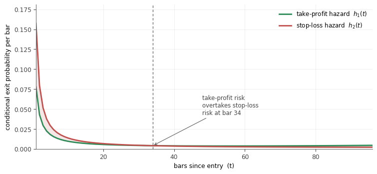
Fig. 2. Cause-specific hazards from the real fitted XAUUSD model, evaluated at mean covariate values. Both hazards fall steeply from bar 1 rather than peaking mid-window — most trades that are going to hit a barrier do so quickly, and the ones that survive longer are increasingly likely to be range-bound. Take-profit risk overtakes stop-loss risk around bar 34, simply because the stop-loss hazard decays faster from a higher starting point, not because it rises.

That shape was not what an earlier synthetic test of this fitting code had suggested (a mid-window hump) — the true shape only shows up once real data is fitted, a reminder not to over-trust a model's behaviour on simulated inputs before checking it against the real thing.

From cumulative incidence to an exit decision

Hazards are not yet a decision. To act, roll them forward from the current bar to the time stop, accumulating cumulative incidence for each cause and the residual probability of still being open at the end:

void CCompetingRisks::PredictCIF(const int t_start, const double &x[],
                                 double &cifTP, double &cifSL, double &survOpen) const
  {
   cifTP = 0.0;
   cifSL = 0.0;
   double S = 1.0;
   for(int s = MathMax(t_start, 1); s <= m_tmax; s++)
     {
      double h1, h2;
      Hazards(s, x, h1, h2);
      cifTP += h1 * S;
      cifSL += h2 * S;
      S     *= MathMax(0.0, 1.0 - h1 - h2);
     }
   survOpen = S;
  }

Covariates are held constant during the projection. This is a last-value-carried-forward approximation. But the position is rescored every new bar, so any projection is used for exactly one bar before being replaced.

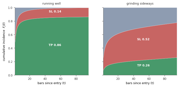
Fig. 3. Cumulative incidence from the real XAUUSD model for two contrasting, illustrative covariate profiles at identical trade age. A trade running well (strong MFE, small MAE, in profit) finishes at target 86% of the time under this fitted model; a trade grinding sideways with little MFE finishes at target only 26% of the time and is still open at the time stop 22% of the time.

The decision is now arithmetic. Reaching the target pays R TP , the stop costs exactly one R by construction, and a trade still open at the time stop settles at roughly its current R:

E[hold] = π TP · R TP − π SL · 1.0 + π open · R now

E[close] = R now

Close early when E[hold] < E[close] − δ. Without the margin, the rule fires every time the two expectations cross on noise, and you pay the spread for it.

A second rule catches what the expected-value comparison handles sluggishly: when the stop-loss hazard runs well above the take-profit hazard on a position in profit, the trade has turned even before the expectations cross.

double e_hold  = cifTP * g_rtp - cifSL * 1.0 + sOpen * cur_R;
double e_close = cur_R;

if(g_state.bars_held < InpMinHold)
   return;

//--- Rule 1: holding is no longer worth what closing is worth.
bool close_now = (e_hold < e_close - InpEdgeDelta);

//--- Rule 2: the trade has turned while still in profit.
if(!close_now && cur_R > 0.0 && h1 > 1e-9)
   close_now = ((h2 / h1) > InpHazardRatio);

The hard take-profit and stop-loss orders stay on the position throughout. The model only ever closes early. As Section 7 shows, that bound did not stop the policy from underperforming on two of the four instruments tested — reducing exposure is not automatically the same as improving outcomes.

The two threshold parameters, InpEdgeDelta and InpHazardRatio, were not refit per instrument — held at 0.02 and 2.5 everywhere, deliberately, for reproducibility. That choice matters more than expected, discussed once the real results are on the table.

The live decision is rendered on the chart by SurvivalPanel.mqh, a small CCanvas bitmap label that turns the four numbers PredictCIF() just produced into something readable at a glance:

void CSurvivalPanel::Update(const bool has_pos, const int bars_held, const int tmax,
                            const double cur_R, const double cifTP, const double cifSL,
                            const double sOpen, const double e_hold, const double e_close,
                            const double h1, const double h2)
  {
   if(!m_ok)
      return;
   m_c.Erase(Argb(clrBlack, 190));

   //--- Stacked incidence bar: green width proportional to cifTP, red to cifSL.
   int bx = 10, by = 56, bw = m_w - 20, bh = 22;
   int wTP = (int)MathRound(bw * MathMax(cifTP, 0.0));
   int wSL = (int)MathRound(bw * MathMax(cifSL, 0.0));
   m_c.FillRectangle(bx, by, bx + wTP, by + bh, Argb(clrMediumSeaGreen));
   m_c.FillRectangle(bx + wTP, by, bx + wTP + wSL, by + bh, Argb(clrIndianRed));

   color ec = (e_hold >= e_close ? clrMediumSeaGreen : clrOrange);
   m_c.TextOut(10, 166, StringFormat("E[hold] %+.3f   E[close] %+.3f", e_hold, e_close), Argb(ec));
   m_c.Update();
  }

The colour on the expected-value line is the useful part: green while holding is worth more than closing, orange the moment that flips. The panel is created only when InpShowPanel and MQL_VISUAL_MODE are true. Otherwise, the Strategy Tester would not render the bitmap.

Edge cases and pitfalls

SYMBOL_TRADE_TICK_VALUE can be wrong for JPY-quoted pairs. Position sizing was originally built from SYMBOL_TRADE_TICK_VALUE / SYMBOL_TRADE_TICK_SIZE directly. On USDJPY, on the broker used here, that property reported a tick value of 100.00 — roughly 160 times too large. The position size silently rounded to the broker's 0.01 minimum lot, and every trade risked about 1/40th of the intended 1% with no warning, caught only because the average loss ($2.41) was implausibly small next to the other three instruments ($44–$84). The fix is OrderCalcProfit(), which asks the terminal what a hypothetical trade would gain or lose and is guaranteed to agree with the engine that executes it:

double loss_for_1_lot = 0.0;
ENUM_ORDER_TYPE ot = (dir > 0 ? ORDER_TYPE_BUY : ORDER_TYPE_SELL);
if(!OrderCalcProfit(ot, _Symbol, 1.0, price, sl, loss_for_1_lot) || loss_for_1_lot >= 0.0)
  {
   PrintFormat("LotsForRisk: OrderCalcProfit failed - falling back to InpLots.");
   return(InpLots);
  }
double lots = (AccountInfoDouble(ACCOUNT_BALANCE) * InpRiskPercent / 100.0) / MathAbs(loss_for_1_lot);

If sizing positions from a risk percentage on more than one instrument, verify this by eye once: check that the average loss per trade in the tester report is a sane multiple of the intended risk. A silent 40x undersizing still produces a report that runs and looks superficially plausible.

Field-based CSV reading proved unreliable; line-based reading did not. An earlier build of SurvivalModelTrainer.mq5 's reader used FileReadNumber()/FileIsLineEnding() to parse the CSV field by field. In testing that dropped 60–86% of rows depending on the exact variant, and the corruption pattern shifted with every fix attempted rather than resolving. The final fix is applied on both ends. The writer formats each field explicitly before calling FileWrite(). The reader parses whole lines with StringSplit() instead of relying on CSV field mode. Every dataset behind Section 7's results table loaded with zero rejected rows this way.

//--- Each field is written as an explicitly self-formatted string, passed
//--- to FileWrite as its OWN argument. Separate arguments let FILE_CSV
//--- mode place the delimiter correctly - a single hand-joined string
//--- does not round-trip reliably. And pre-formatting with
//--- IntegerToString/DoubleToString - both always period-decimal
//--- regardless of the terminal's Windows region - denies MQL5 any
//--- chance to render 0.78 as "0,78" on a comma-decimal locale, which
//--- would silently split into two fields against the comma delimiter.
for(int i = 0; i < nrows; i++)
  {
   FileWrite(fh,
            IntegerToString(rows[i].trade_id),
            IntegerToString((long)rows[i].entry_time),
            IntegerToString(rows[i].t),
            IntegerToString(rows[i].y),
            DoubleToString(rows[i].x[0], 8), DoubleToString(rows[i].x[1], 8),
            DoubleToString(rows[i].x[2], 8), DoubleToString(rows[i].x[3], 8),
            DoubleToString(rows[i].x[4], 8), DoubleToString(rows[i].x[5], 8),
            DoubleToString(rows[i].x[6], 8), DoubleToString(rows[i].x[7], 8),
            DoubleToString(rows[i].x[8], 8));
  }

The header row's column count is derived from the feature contract rather than typed as a literal 13, so a change to SURV_NUM_FEATURES shows up in the file the very next run instead of quietly writing the wrong number of columns:

//--- Header. Column count is derived from the contract, never typed out.
string hdr = "trade_id,entry_time,t,y";
for(int k = 0; k < SURV_NUM_FEATURES; k++)
   hdr += "," + CSurvivalFeatures::Name(k);
FileWrite(fh, hdr);

A model does not transfer between symbols. The coefficients encode how one market's state maps to barrier-hit probability, and the standardisation constants are that symbol's own means and deviations. Each instrument needs its own build-and-train pass. Check holdout improvement over the time-only baseline per instrument before trusting an exit rule — all four instruments here cleared 20%.

Calibration transferring does not mean the decision rule transfers. The central finding of this article: the hazard model calibrated well on every instrument, but fixed thresholds built on it did not produce a consistent trading improvement. A well-calibrated probability and a well-tuned decision threshold are different things.

Both barriers inside one bar. M30 bars can span more than a one-ATR stop distance. Tick data would resolve the ordering; the harvester assumes the stop printed first — biasing the take-profit hazard slightly downward, the safe direction.

The Strategy Tester sandbox. Each tester agent gets its own MQL5\Files directory, so a manifest written locally is invisible to the backtest. Both artifacts go to the common folder via FILE_COMMON, or the EA fails to initialise in the tester while working fine on a live chart.

SurvivalModelTrainer.mq5's split has to be by trade, not by row. A random row-level split would put periods of the same trade on both sides, and since consecutive periods share nearly identical covariates and the trade's eventual outcome, the holdout would score itself. The split is done on trade ID instead, using the highest ID seen and the leading InpTrainShare fraction of it:

//--- Chronological split by trade, never by row. Splitting rows at
//--- random would put periods of the same trade on both sides and
//--- leak the outcome straight into the holdout.
int max_id = 0;
for(int i = 0; i < g_rows; i++)
   max_id = MathMax(max_id, g_ID[i]);
int cut_id = (int)MathRound(max_id * InpTrainShare);

int ntr = 0, nho = 0;
for(int i = 0; i < g_rows; i++)
  {
   if(g_ID[i] <= cut_id)
      ntr++;
   else
      nho++;
  }

Because trade IDs are assigned in the order the harvester walks the chart, a trade-ID cut is also a time cut — training is every trade opened before some date, holdout is everything after. That is what makes the holdout log-loss a genuine out-of-sample number.

The reader itself is the other half of the CSV fix described above — plain-text lines split with StringSplit() rather than field-mode CSV reads, with a header-column check and a per-row rejection counter so a malformed file fails loudly instead of silently training on fewer rows than it should:

while(!FileIsEnding(fh))
  {
   string line = FileReadString(fh);
   if(StringLen(line) == 0)
      continue;                            // blank line (e.g. trailing EOF line)

   string parts[];
   int n = StringSplit(line, ',', parts);

   if(n != ncol)
     {
      rej_total++;
      continue;
     }

   int    id = (int)StringToInteger(parts[0]);
   int    t  = (int)StringToInteger(parts[2]);
   int    y  = (int)StringToInteger(parts[3]);

   bool bad = (t <= 0 || y < 0 || y > 2);
   for(int k = 0; k < SURV_NUM_FEATURES; k++)
     {
      double v = StringToDouble(parts[4 + k]);
      if(!MathIsValidNumber(v))
         bad = true;
      g_X[g_rows * SURV_NUM_FEATURES + k] = v;
     }
  }

Every dataset used for the table in Section 7 loaded through this reader with zero rejected rows, confirmed against the row counts SurvivalDatasetBuilder.mq5 reported at write time.

Testing in the Strategy Tester

The test design is worth copying even if you never use survival analysis. For each instrument, two runs with identical entry logic, risk and data — only InpExitMode differs. Because entries are byte-identical, the difference between the two equity curves is the exit policy and nothing else.

One instrument proves nothing, so this protocol runs across four instruments spanning two market types — three major currency pairs and a metal — with every input below held identical.

Setting	Value
Instruments	EURUSD, GBPUSD, USDJPY, XAUUSD — all M30
Entry (both arms)	20-bar Donchian breakout, ATR(14) above its 100-bar median
Stop / target / time stop	1.0 × ATR(14) / 2.0 R / 96 bars
Dataset window (builder)	2023.01.01 – 2025.06.30, InpFrom/InpTo identical on every symbol
Train / holdout split	InpTrainShare = 0.60, chronological by trade ID
Ridge λ / iterations / tolerance	1.0 / 25 / 1e-7
Strategy Tester date range	2024.07.01 – 2025.06.30 (the holdout period only)
Modelling	1 Minute OHLC
Position sizing	1% of balance per trade via OrderCalcProfit, identical on every instrument
Edge margin δ / hazard ratio / min hold	0.02 / 2.5 / 2 bars, identical on every instrument
Deposit	10,000 USD

The Strategy Tester date range is deliberately the holdout period only — running the backtest over training data too would not be out-of-sample. The builder's window, trainer's split, and tester's date range all have to agree. Fig. 4 shows two real calibration checks from the actual runs behind the table below:

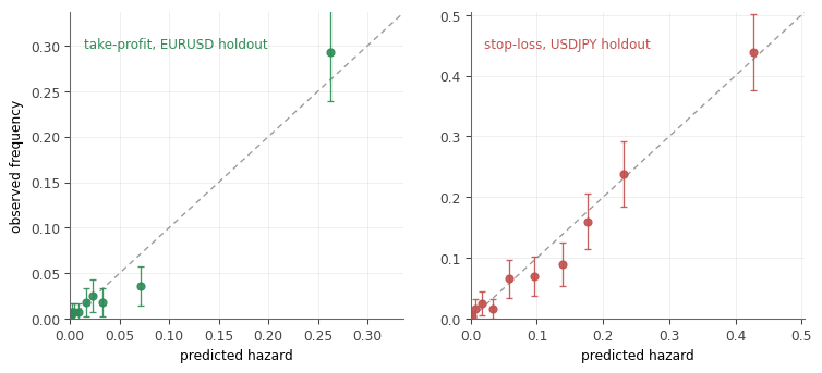
Fig. 4. Holdout decile calibration from two of the four real fits, with 95% intervals. Points on the diagonal mean predicted probabilities can be taken at face value. Both panels track the diagonal closely through the upper deciles, which is what the 20–22% log-loss improvement in the table above looks like in calibration terms.

Instrument	Exits	Trades	Net profit	Profit factor	Expected payoff	Max drawdown	Win rate	Sharpe
EURUSD	fixed	464	-6,841.94	0.64	-14.75	70.28%	25.22%	-5.00
EURUSD	survival	508	-6,212.69	0.59	-12.23	62.49%	32.87%	-5.00
GBPUSD	fixed	467	-3,995.86	0.85	-8.56	46.51%	29.98%	-3.68
GBPUSD	survival	515	-3,401.17	0.84	-6.60	40.16%	35.53%	-5.00
USDJPY	fixed	452	-3,614.99	0.86	-8.00	41.67%	30.31%	-3.20
USDJPY	survival	507	-4,293.61	0.77	-8.47	46.74%	32.94%	-5.00
XAUUSD	fixed	469	-1,379.40	0.95	-2.94	30.23%	32.62%	-1.09
XAUUSD	survival	507	-3,012.58	0.83	-5.94	35.33%	33.33%	-4.56
All four, fixed	—	1,852	-15,832.19	0.84	—	47.2% avg	29.5%	-3.24 avg
All four, survival	—	2,037	-16,920.05	0.77	—	46.2% avg	33.7%	-4.89 avg

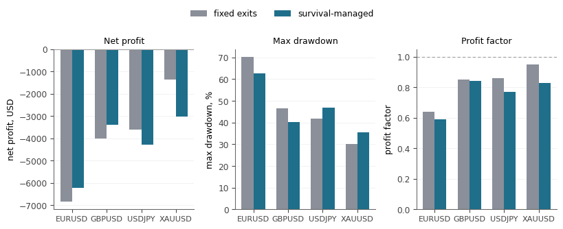
Fig. 5. Net profit, max drawdown and profit factor, fixed against survival-managed exits, all four instruments, real Strategy Tester output. No column improves on every instrument; profit factor is worse under survival exits on all four.

First, the entries. Both arms lose money on every instrument — the Donchian breakout filter used here is weak over this eighteen-month window, roughly a third take-profit to two-thirds stop-loss on every symbol, and no exit policy fixes a bad entry signal. That was expected and is not the finding of this article.

The finding is in how the two exit policies compare, and it does not support a simple "the model helps" headline. Profit factor is worse under survival exits on all four instruments, and Sharpe on three of four. Win rate improves everywhere — survival exits convert some fraction of eventual losers into smaller, more frequent trades. A higher win rate bought at a worse profit factor is not obviously a good trade.

Net profit and drawdown split cleanly by how bad the fixed-exit baseline already was. On EURUSD and GBPUSD — worst fixed-arm profit factors, 0.64 and 0.85 — survival exits reduced dollar loss and drawdown. On USDJPY and XAUUSD — best fixed-arm profit factors, 0.86 and 0.95 — survival exits made both worse, and on XAUUSD the loss more than doubled. In aggregate, survival exits lost more money ($16,920 vs $15,832) with a worse profit factor (0.77 vs 0.84).

The hazard model and the decision rule are separate claims. This test validates only the model. Every diagnostics number in Section 4 says the model calibrates reliably: 20–22% log-loss improvement on every instrument, deciles tracking the diagonal in Fig. 4. What does not transfer is InpEdgeDelta and InpHazardRatio held at the same value everywhere — a margin protecting a badly losing system may simply cut into upside on a system already closer to breakeven. This test held those thresholds fixed for reproducibility, and the reproducible result is that fixed thresholds are not a free improvement.

This is the useful shape of a real result: not "always works", not "never works", but a falsifiable claim — the probability model transfers across instruments, a fixed decision rule on top of it does not, and the next test is whether per-instrument threshold tuning recovers what a single global threshold gave up.

Conclusion

A trade that is still open is an observation, not a pending verdict — having survived this far is itself information. Discrete-time competing risks writes that down honestly: two hazards competing for one trade, a cumulative incidence that respects the competition, and censoring handled by rows that stop appearing rather than a fudge factor.

The implementation turned out lighter than expected. A multinomial logit on a person-period table is an ordinary Newton-Raphson problem, and the native matrix type handles 24 parameters comfortably. Keeping it inside MQL5 lets the training and live paths share one covariate builder.

The cross-instrument test is where this article earns its conclusions rather than assuming them. Four instruments, identical entry logic, risk sizing and exit thresholds, only the exit policy toggled. The hazard model calibrated consistently everywhere — a real, reproducible result. The trading outcome from a fixed decision rule built on it did not: it helped on the two weakest baselines, hurt on the two strongest, and lost more money than doing nothing extra averaged across all four.

The most promising next step follows directly from that gap: fit InpEdgeDelta and InpHazardRatio per instrument instead of globally, using the same holdout split already in the trainer, and see whether tuning recovers what a shared threshold gave up on USDJPY and XAUUSD. A second direction replaces the fixed take-profit with a model-chosen one.

Whatever you build on top, keep the two-arm test design and report every instrument tested, not only the ones that flatter the method. Holding entries fixed while varying only the exit is the cleanest attribution available, and it is only informative if the full spread of results — including the two that went the wrong way — makes it into the write-up.

File	Type	Description
TradeSurvivalExitEA.mq5	Expert Advisor	Donchian entries with selectable fixed or survival-managed exits. Loads the manifest for its own symbol and timeframe, sizes positions via OrderCalcProfit, and scores every open position on each new bar against both decision rules.
SurvivalFeatures.mqh	Include	The feature contract: the nine time-varying covariates, the shared series cache both the harvester and the live EA read through, and the self-test every component runs before touching the market.
CompetingRisks.mqh	Include	Newton-Raphson multinomial fit, cause-specific hazards, cumulative incidence, and manifest read/write, keyed by symbol and timeframe.
SurvivalHarvest.mqh	Include	The shared entry rule, virtual-trade replay, and the person-period expansion that turns historical bars into the estimation table.
SurvivalPanel.mqh	Include	A CCanvas bitmap panel rendering live cumulative incidence and the hold-versus-close comparison on the chart, visual-mode only.
SurvivalDatasetBuilder.mq5	Script	Replays the sample window and writes survival_dataset_<SYMBOL>_<PERIOD>.csv to the common folder, one field per FileWrite argument, self-formatted to a fixed decimal point regardless of the terminal's Windows region. Run once per instrument.
SurvivalModelTrainer.mq5	Script	Reads the CSV as plain text with StringSplit, fits on a chronological trade-level split, reports holdout log-loss and decile calibration against a time-only baseline, writes survival_model_<SYMBOL>_<PERIOD>.mft. Run once per instrument.