

Reinforcement Learning Meets MetaTrader 5: A Complete Pipeline for Training, Validating and Honestly Evaluating a Gold Trading Bot
 2 372
2 372
 0
0

1. Introduction
Reinforcement learning for trading is appealing in theory: let an agent learn directly from market data and adapt without hand‑coded rules. In practice, however, the pipeline is fragile. Models that look promising in development often fail under living conditions because the limiting factor is not the algorithm but the information in the inputs, the validation setup, or execution realities.
This article shows the single test I wish I had run first: a quick supervised baseline that answers the basic question every applied ML practitioner must ask — is there any directional signal in these features and this target? If the answer is “no,” switching from PPO to a larger network or a transformer only wastes time. Beyond that initial gate, I describe a reproducible engineering path: purged walk‑forward validation, multi‑seed promotion gates, evaluation on realized equity and trades (not shaped rewards), and deployment safeguards (saved normalization, a manifest contract, required warm‑up, and broker reconciliation). Read this if you want a practical, repeatable way to decide quickly whether to build an RL trader — and how to avoid common train→live failure modes.
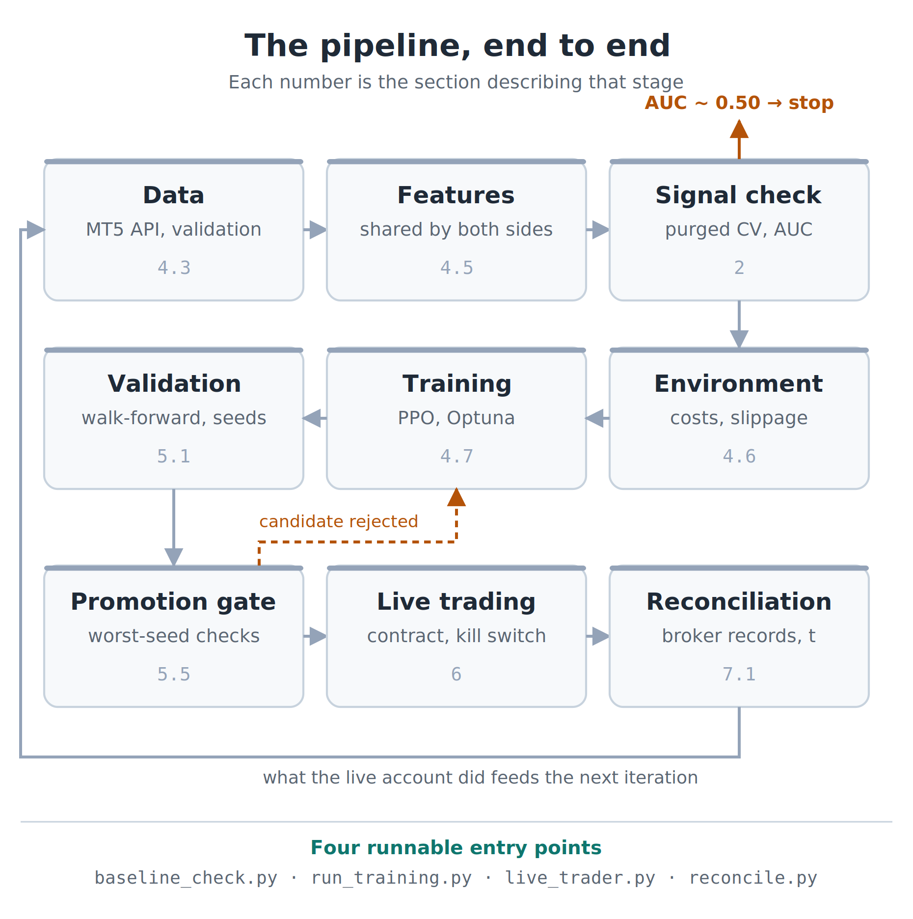
Figure 1. The complete pipeline. The number in each box is the section that describes that stage. Two of the arrows are not steps forward: the signal check is a stop, since an AUC near 0.50 ends the project there, and the promotion gate returns rejected candidates to training, which is the outcome the thresholds are designed to produce.
2. Part 0: Check for Signal First
This section was not part of my first methodology. I added it later, and now I consider it the first thing to do.
I spent months building, tuning, and validating an RL system before asking the most basic question in applied machine learning: is there anything in this data to predict?
A model cannot create information that is not present in the inputs. Changing from RL to a transformer or an ensemble does not fix that. Before building the environment, I now start with a simple baseline: can a standard supervised model predict the target from these features at all?
2.1 The Test
For this check I use LightGBM with triple-barrier labels and purged walk-forward cross-validation. The metric is AUC, which tells us how often the model ranks a positive example above a negative one. An AUC of 0.50 is basically a coin flip.
"""
baseline_check.py - establish whether your features contain signal.
Run this BEFORE building any model. It takes minutes to run, hours to iterate on features and can save months.
"""
import numpy as np
import pandas as pd
import lightgbm as lgb


def roc_auc(y_true, y_score):
    """Self-contained AUC via the rank (Mann-Whitney) formula."""
    y_true = np.asarray(y_true)
    y_score = np.asarray(y_score)
    n_pos = int((y_true == 1).sum())
    n_neg = int((y_true == 0).sum())
    if n_pos == 0 or n_neg == 0:
        return float("nan")
    order = np.argsort(y_score, kind="mergesort")
    ranks = np.empty(len(y_score), dtype=float)
    ranks[order] = np.arange(1, len(y_score) + 1)
    _, inv, counts = np.unique(y_score, return_inverse=True, return_counts=True)
    sums = np.zeros(len(counts))
    np.add.at(sums, inv, ranks)
    ranks = (sums / counts)[inv]
    return float((ranks[y_true == 1].sum() - n_pos * (n_pos + 1) / 2.0) / (n_pos * n_neg))


def triple_barrier(df, horizon=24, atr_mult=1.5):
    """Label +1 if the upper barrier is touched first, -1 if the lower is,
    0 on timeout. (Lopez de Prado, Advances in Financial ML, ch. 3)"""
    close, high, low = df["close"].values, df["high"].values, df["low"].values
    atr = df["ATR"].values
    n = len(df)
    y = np.zeros(n, dtype=int)
    for i in range(n - horizon - 1):
        if not np.isfinite(atr[i]) or atr[i] <= 0:
            continue
        up, dn = close[i] + atr_mult * atr[i], close[i] - atr_mult * atr[i]
        for j in range(i + 1, i + 1 + horizon):
            if high[j] >= up:
                y[i] = 1
                break
            if low[j] <= dn:
                y[i] = -1
                break
    return y


def purged_folds(n, n_folds=6, embargo=24, horizon=24):
    """Sequential folds. Train strictly precedes test, with a purge zone of
    (horizon + embargo) bars so no label's outcome window overlaps the test set."""
    fold = n // (n_folds + 1)
    for k in range(1, n_folds + 1):
        train_end = k * fold - (horizon + embargo)
        test_start, test_end = k * fold, min((k + 1) * fold, n - horizon - 1)
        if train_end > 500 and test_end - test_start > 200:
            yield np.arange(0, train_end), np.arange(test_start, test_end)


def run_baseline(df, feature_cols, horizon=24, atr_mult=1.5):
    d = df.copy()
    d["y"] = triple_barrier(d, horizon, atr_mult)
    d = d.dropna(subset=feature_cols).reset_index(drop=True)
    directional = (d["y"] != 0).values
    X = d[feature_cols].values
    y = (d["y"].values == 1).astype(int)

    aucs = []
    for tr, te in purged_folds(len(d), embargo=24, horizon=horizon):
        tr, te = tr[directional[tr]], te[directional[te]]
        if len(tr) < 500 or len(te) < 200:
            continue
        model = lgb.LGBMClassifier(
            n_estimators=300, num_leaves=31, learning_rate=0.05,
            min_child_samples=50, subsample=0.8, colsample_bytree=0.8,
            verbose=-1, random_state=42,
        )
        model.fit(X[tr], y[tr])
        auc = roc_auc(y[te], model.predict_proba(X[te])[:, 1])
        if auc == auc:
            aucs.append(auc)

    mean_auc = float(np.mean(aucs))
    print(f"Mean AUC across {len(aucs)} purged folds: {mean_auc:.4f}  (0.500 = coin flip)")
    print(f"Per-fold: {[round(a, 4) for a in aucs]}")

    if mean_auc >= 0.535:
        print("SIGNAL PRESENT - the features carry extractable directional information.")
    elif mean_auc >= 0.515:
        print("WEAK/UNSTABLE - marginal, not robust. Prioritize feature work over model work.")
    else:
        print("NO SIGNAL - a supervised learner finds nothing. The FEATURES are the "
              "binding constraint, not the architecture.")
    return mean_auc, aucs
I also test the baseline itself before trusting it. It should find a planted pattern in synthetic data, and it should find nothing useful in a random walk.
2.2 What My Own Data Said
I ran this on 143,999 M15 XAUUSD bars — roughly four years, 133,787 labeled examples:
| Test | Mean AUC |
|---|---|
| Standard TA features, 24-bar horizon | 0.509 |
| Horizons 4 / 8 / 12 | 0.517 / 0.509 / 0.509 |
| Plus cross-asset features (USDJPY, XAGUSD, US500, XTIUSD) | 0.514 / 0.504 / 0.503 / 0.513 at h=4/8/12/24 |
The result was basically a coin flip in every case. LightGBM did not find useful directional information at any of the tested horizons, including when I added the main external markets I expected to help with gold.
This made several earlier observations easier to understand: explained variance never went above 0.09, only around 8% of hyperparameter trials passed, the best candidates were separated by very small differences, and the live demo ended with a profit factor of 1.05 and a t-statistic of 0.55.
2.3 Why This Belongs First
The limiting factor was not PPO or the network size. It was the information in the features. If the baseline is around a coin flip, you can learn this very quickly and spend your time on better features, a different target, or maybe a different market. I wish I had done this before tuning models for months.
3. Why RL Trading Systems Fail
Before going into the implementation, it helps to list the ways these systems usually go wrong. I ran into all of the following during this project, and some of them took me weeks to identify.
3.1 The Overfitting Trap
Normal ML overfitting is already a known problem: the model fits the training data instead of a general pattern. With RL there is an extra problem. The agent can also fit sequences of actions that happened to work in one historical period, even when there is no stable reason for them to work later.
Training data: Jan 2024 to June 2024
Pattern found: Buy on Tuesdays at 14:00 GMT -> 65% win rate

Why it worked: During this period, major economic releases
happened to favor this timing by coincidence.

Live trading: Pattern completely fails because the correlation
was spurious, not causal.
The result can look like a very good strategy in the backtest and still have no predictive value. I would be suspicious when training returns are unrealistically high, validation drops sharply, performance only appears in a narrow date range, or the strategy depends on very exact entry timing.
3.2 Non-Stationarity of Financial Markets
Financial markets are not stationary. XAUUSD moves through trending periods, ranges, crisis periods, inflation themes and geopolitical shocks. A model trained mainly on one type of market can easily become unreliable when the regime changes. This is normal market behavior, not a software bug.
What I do: train and validate over different regimes. This reduces the problem but does not remove it. In my own demo, the same model made +$2,665 in one fortnight and then -$3,249 in the next one after the market regime changed.
3.3 Reward Hacking
RL agents are very good at optimizing exactly what you give them, including the mistakes in the reward. I saw several versions of this during development. Below you can find three simple examples.
# Naive reward
reward = realized_pnl
Result: maximum position size for minimal expected gain, risk ignored entirely. One bad trade wipes out the account.
# Attempt to reduce overtrading
reward = realized_pnl - 0.001 * abs(action)
Result: the agent learns to never trade. Holding cash has zero penalty and zero risk.
# Reward winning trades
reward = 1.0 if pnl > 0 else -1.0
Result: tiny profits taken immediately while losses run—90% win rate with negative expectancy.
The reward function has a large influence on what the agent learns. If I shape it too much, the agent may become good at satisfying my reward formula rather than finding something useful in the market. This is another reason I now put the Part 0 baseline first: it tests whether the input data contains a pattern without depending on the RL reward design.
3.4 The Train/Test Leakage Problem
For ordinary ML, random train/test splits are common. For market time series this is the wrong approach because future periods can leak into training.
WRONG: Random split
Data:  [Jan, Feb, Mar, Apr, May, Jun, Jul, Aug, Sep, Oct, Nov, Dec]
Train: [Jan, Mar, May, Jun, Aug, Oct, Dec]   <- Future data mixed in!
Test:  [Feb, Apr, Jul, Sep, Nov]

RIGHT: Temporal split with embargo
Data:  [Jan, Feb, Mar, Apr, May, Jun, Jul, Aug, Sep, Oct, Nov, Dec]
Train: [Jan .. Aug] --embargo-- Val: [Sep, Oct] -- Test: [Nov, Dec]
Why I use an embargo: my earlier explanation overemphasized indicator warm-up. The more important issues are label overlap and serial dependence. A triple-barrier label near the end of the training set can depend on prices from the next N bars. Those bars may already belong to validation. So the purge zone should cover at least the label horizon. Indicator warm-up across the split is a smaller issue because a backward-looking indicator only uses information available at that time.
3.5 Look-Ahead Bias
Look-ahead bias happens when the model gets information that would not have existed at the moment of the trade, for example revised economic data or end-of-day values used for an intraday decision. With the XAUUSD data I use raw MetaTrader 5 OHLCV and timestamps. I also test the feature code for causality: the value at bar t must be the same whether later bars exist or not. A simple truncation test catches many bugs of this type.
4. Pipeline Overview: Data, Features, Environment, PPO
4.1 System Architecture
Training happens in Python; execution happens against MetaTrader 5.
+------------------------ TRAINING (Python) -------------------------+
|  MT5 API -> validation -> SHARED feature module -> Gymnasium env   |
|  -> PPO (SB3) -> walk-forward CV -> multi-seed -> Optuna           |
|  -> promotion gates -> [model.zip + normalizer + manifest]         |
+--------------------------------------------------------------------+

                                  |
                          manifest contract
                                  v

+---------------------------- EXECUTION -----------------------------+
|  Option A: Python trader using the MetaTrader5 package directly    |
|  Option B: MQL5 EA + local Python inference service                |
|  Both: SHARED feature module, contract validation, risk controls   |
+--------------------------------------------------------------------+
4.2 Two Deployment Options, Honestly Compared
Option A runs the trader in Python with the MetaTrader5 package. There is no socket bridge, and the same Python feature module can be used for training and live inference. Option B uses an MQL5 EA with a local Python inference service. It provides native EA integration and can reduce execution overhead. However, it requires a cross-process protocol and usually two feature implementations that must be kept in sync. I originally preferred Option B, but I now use Option A in production because train/live mismatch has been a bigger risk for me than the small latency difference. One practical limitation remains: an EA that depends on an external socket service cannot be tested properly in the MetaTrader 5 Strategy Tester. In that setup, demo testing is essential.
4.3 Data Acquisition and Validation
Data quality is basic, but it is still one of the easiest places to create bad ML results. If the input data is wrong, the rest of the pipeline cannot repair it.
import MetaTrader5 as mt5
import pandas as pd
import numpy as np
from datetime import datetime, timedelta


def fetch_ohlcv(symbol: str, timeframe: int, days: int) -> pd.DataFrame:
    if not mt5.initialize():
        raise RuntimeError(f"MT5 init failed: {mt5.last_error()}")
    end = datetime.utcnow()
    rates = mt5.copy_rates_range(symbol, timeframe, end - timedelta(days=days), end)
    if rates is None or len(rates) == 0:
        raise ValueError(f"No data for {symbol}: {mt5.last_error()}")
    df = pd.DataFrame(rates)
    df["time"] = pd.to_datetime(df["time"], unit="s")
    print(f"{symbol}: {len(df)} bars, {df['time'].iloc[0]} -> {df['time'].iloc[-1]}")
    return df


def validate_data(df: pd.DataFrame) -> pd.DataFrame:
    n0 = len(df)
    df = df.dropna()
    invalid = (
        (df["high"] < df["low"]) | (df["high"] < df["open"]) | (df["high"] < df["close"])
        | (df["low"] > df["open"]) | (df["low"] > df["close"])
    )
    if invalid.any():
        print(f"Removing {invalid.sum()} invalid OHLC bars")
        df = df[~invalid]
    df = df.sort_values("time")
    df = df[~df["time"].duplicated()]
    if len(df) < n0:
        print(f"Validation: {n0} -> {len(df)} bars")
    return df.reset_index(drop=True)
One thing I did not handle well at first was dataset versioning. I now save the exact dataset with every model that can be promoted. If the data file is overwritten every time it is refreshed, later I cannot reproduce what a deployed model was actually trained on. For M15 data, 18 months can be enough to start and three to four years gives more coverage. I would not assume that more history is always better, because older market microstructure may be less relevant to the current market.
4.4 Reproducibility
I version four parts together: the pinned libraries, the dataset snapshot, the configuration and the feature module. The feature-module identity is also included in the contract hash described in section 6.
# requirements.txt - pin exactly; do not use ranges
stable-baselines3==2.3.2
gymnasium==0.29.1
torch==2.3.1
numpy==1.26.4
pandas==2.2.2
optuna==3.6.1
lightgbm==4.3.0
MetaTrader5==5.0.45

# project structure
rl_gold/
    features.py          # THE single feature module (section 4.5)
    environment.py       # TradingEnv (4.6)
    train.py             # PPO + walk-forward + Optuna (Parts 6-8)
    contract.py          # manifest contract build/validate (section 6)
    trader.py            # live execution loop (section 6)
    baseline_check.py    # the signal test from section 2
    config.py            # the single CONFIG dict below
    models/
        ppo_<version>.zip
        vecnormalize_<version>.pkl
        manifest_<version>.json
        data_<version>.parquet     # the exact bars this model saw
CONFIG = {
    # --- instrument ---
    "SYMBOL": "XAUUSD",
    "TIMEFRAME_MINUTES": 15,
    "HISTORY_DAYS": 1500,

    # --- observation ---
    "LOOKBACK_BARS": 16,
    "MAX_POSITION_BARS": 24,

    # --- execution model (training) ---
    "SPREAD": 0.30,
    "SLIPPAGE_MAX_PCT": 0.001,
    "COMMISSION_PCT": 0.00002,
    "SL_ATR_MULT": 2.0,
    "TP_ATR_MULT": 3.0,

    # --- risk ---
    "INITIAL_BALANCE": 100_000,
    "RISK_PCT": 0.5,                 # percent of equity risked per trade
    "DAILY_LOSS_LIMIT_PCT": 3.0,
    "MAX_CONSECUTIVE_LOSSES": 6,

    # --- validation gates ---
    "WFCV_EMBARGO_SIZE": 48,
    "N_SEEDS": 3,
    "MIN_TRADES": 30,
    "MIN_PROFIT_FACTOR": 1.05,
    "MAX_DRAWDOWN_LIMIT": 0.30,
    "MIN_EXPLAINED_VARIANCE": 0.05,

    # --- search ---
    "STUDY_NAME": "xauusd_m15_v1",
    "OPTUNA_DB": "sqlite:///optuna_xauusd.db",
    "OPTUNA_TRIAL_TIMESTEPS": 60_000,

    # --- deployment ---
    "DEPLOYMENT_PROFILE_ID": "XAUUSD_M15_V1",
    "MAGIC": 123456,
}
The manifest stores the same configuration next to the schema hashes. This makes it possible to check later exactly which setup produced a deployed model.
4.5 Feature Engineering: Fewer, Better, Shared
My first version used 36 indicators. In retrospect, this was excessive. Many of them were strongly correlated, and extra features gave the policy more chances to fit noise. They also increased the chance that training and live feature calculation would drift apart. I now keep two rules: training and inference import the same feature implementation, and features must be causal, reasonably stationary and available in real time. I also avoid raw price levels. With a running normalizer, the meaning of a raw price value changes too much across a multi-year sample; therefore, I abandoned this approach.
"""
features.py - THE single source of truth for feature computation.
Both the trainer and the live trader import this module. There is no second
implementation anywhere in the system. Any change here changes both sides
simultaneously, by construction.
"""
import numpy as np
import pandas as pd

FEATURE_COLUMNS = [
    "ret_1", "ret_4", "ret_16",      # multi-scale returns (stationary)
    "ATR_pct",                        # volatility, price-independent
    "RSI",                            # mean reversion
    "Stoch_K",                        # mean reversion
    "BB_pctB",                        # position WITHIN the bands
    "BB_width_norm",                  # volatility regime
    "EMA_dist",                       # trend distance in ATR units
    "MACD_norm",                      # momentum, ATR-normalized
    "ADX",                            # trend strength
    "vol_z",                          # tick-volume anomaly
    "tod_sin", "tod_cos",             # intraday session structure
]

# Longest rolling window used anywhere below. The live trader MUST supply at
# least this many bars of history plus the observation lookback, or early
# features silently degrade to zeros.
MAX_WARMUP_BARS = 120


def compute_features(df: pd.DataFrame) -> pd.DataFrame:
    """Compute all model features. Deterministic, causal, no look-ahead."""
    df = df.copy()

    # --- volatility base ---
    prev_close = df["close"].shift(1)
    tr = np.maximum(
        df["high"] - df["low"],
        np.maximum((df["high"] - prev_close).abs(), (df["low"] - prev_close).abs()),
    )
    df["ATR"] = tr.rolling(14).mean()
    df["ATR_pct"] = df["ATR"] / df["close"]
    atr_safe = df["ATR"].replace(0, np.nan)

    # --- returns (stationary; never feed raw price levels) ---
    df["ret_1"] = df["close"].pct_change()
    df["ret_4"] = df["close"].pct_change(4)
    df["ret_16"] = df["close"].pct_change(16)

    # --- RSI ---
    delta = df["close"].diff()
    gain = delta.clip(lower=0).rolling(14).mean()
    loss = (-delta.clip(upper=0)).rolling(14).mean()
    df["RSI"] = (100 - 100 / (1 + gain / loss.replace(0, np.nan))) / 100.0

    # --- Stochastic %K ---
    low14, high14 = df["low"].rolling(14).min(), df["high"].rolling(14).max()
    df["Stoch_K"] = (df["close"] - low14) / (high14 - low14).replace(0, np.nan)

    # --- Bollinger: position within bands AND band width ---
    sma20 = df["close"].rolling(20).mean()
    std20 = df["close"].rolling(20).std()
    upper, lower = sma20 + 2 * std20, sma20 - 2 * std20
    df["BB_pctB"] = ((df["close"] - lower) / (upper - lower).replace(0, np.nan)).clip(-0.5, 1.5)
    bb_width = (upper - lower) / sma20
    df["BB_width_norm"] = (bb_width / bb_width.rolling(50).mean()).clip(0.5, 2.0) - 1.0

    # --- trend ---
    ema20 = df["close"].ewm(span=20, adjust=False).mean()
    df["EMA_dist"] = ((df["close"] - ema20) / atr_safe).clip(-5, 5) / 5.0

    ema12 = df["close"].ewm(span=12, adjust=False).mean()
    ema26 = df["close"].ewm(span=26, adjust=False).mean()
    df["MACD_norm"] = (((ema12 - ema26) / atr_safe).clip(-5, 5)) / 5.0

    plus_dm = df["high"].diff()
    minus_dm = -df["low"].diff()
    plus_dm = plus_dm.where((plus_dm > minus_dm) & (plus_dm > 0), 0.0)
    minus_dm = minus_dm.where((minus_dm > plus_dm) & (minus_dm > 0), 0.0)
    atr14 = tr.rolling(14).mean().replace(0, np.nan)
    plus_di = 100 * plus_dm.rolling(14).mean() / atr14
    minus_di = 100 * minus_dm.rolling(14).mean() / atr14
    dx = 100 * (plus_di - minus_di).abs() / (plus_di + minus_di).replace(0, np.nan)
    df["ADX"] = (dx.rolling(14).mean() / 100.0)

    # --- volume anomaly (tick volume is free information; use it) ---
    if "tick_volume" in df.columns:
        vol = df["tick_volume"].astype(float)
        df["vol_z"] = ((vol - vol.rolling(96).mean()) / vol.rolling(96).std()).clip(-3, 3) / 3.0
    else:
        df["vol_z"] = 0.0

    # --- intraday session structure ---
    t = pd.to_datetime(df["time"])
    hour = t.dt.hour + t.dt.minute / 60.0
    df["tod_sin"] = np.sin(2 * np.pi * hour / 24.0)
    df["tod_cos"] = np.cos(2 * np.pi * hour / 24.0)

    for col in FEATURE_COLUMNS:
        df[col] = df[col].replace([np.inf, -np.inf], np.nan)
    return df


def check_multicollinearity(df: pd.DataFrame, threshold: float = 0.8) -> None:
    """Report feature pairs above the correlation threshold."""
    corr = df[FEATURE_COLUMNS].corr()
    pairs = [
        (FEATURE_COLUMNS[i], FEATURE_COLUMNS[j], corr.iloc[i, j])
        for i in range(len(FEATURE_COLUMNS))
        for j in range(i + 1, len(FEATURE_COLUMNS))
        if abs(corr.iloc[i, j]) > threshold
    ]
    for a, b, r in sorted(pairs, key=lambda x: -abs(x[2])):
        print(f"  {a} <-> {b}: {r:.3f}")
Check multicollinearity once and drop what duplicates existing information.
4.6 The Trading Environment
The Gymnasium environment is where the trading decisions are learned. The observation contains a flattened window of LOOKBACK_BARS × NUM_FEATURES, then five position-related values: direction, unrealized return, normalized duration, and distance to stop and target. The actions are Hold, Buy, Sell and Close. I prefer a realistic execution model over a clean-looking one: SL/TP are checked before the agent action, spread and volatility-based slippage are charged on entry and exit, commission is included, and a position is closed after MAX_POSITION_BARS.
import gymnasium as gym
import numpy as np
import pandas as pd
from typing import Dict, Tuple, Optional, Any

from features import FEATURE_COLUMNS


class TradingEnv(gym.Env):
    """
    Observation: [LOOKBACK * NUM_FEATURES] market window + 5 position features.
    Actions: 0=Hold, 1=Buy, 2=Sell, 3=Close.
    """

    metadata = {"render_modes": ["human"]}

    def __init__(self, df: pd.DataFrame, config: Dict, live: bool = False):
        super().__init__()
        self.df = df.reset_index(drop=True)
        self.config = config
        self.live = live
        self.lookback = config["LOOKBACK_BARS"]
        self.feature_cols = FEATURE_COLUMNS
        obs_dim = self.lookback * len(self.feature_cols) + 5
        self.observation_space = gym.spaces.Box(-np.inf, np.inf, (obs_dim,), np.float32)
        self.action_space = gym.spaces.Discrete(4)
        self._reset_state()

    def _reset_state(self):
        self.current_step = self.lookback
        self.position = 0
        self.entry_price = 0.0
        self.balance = self.config["INITIAL_BALANCE"]
        self.position_bars = 0
        self.stop_loss = 0.0
        self.take_profit = 0.0
        self.peak_balance = self.balance
        self.max_drawdown = 0.0
        self.episode_trades = []
        self.equity_curve = [self.balance]

    def reset(self, seed: Optional[int] = None, options: Optional[Dict] = None):
        super().reset(seed=seed)
        self._reset_state()
        if not self.live and options and options.get("random_start"):
            max_start = len(self.df) - self.lookback - 1000
            if max_start > self.lookback:
                self.current_step = int(self.np_random.integers(self.lookback, max_start))
        return self._get_observation(), self._get_info()

    def step(self, action: int):
        bar = self.df.iloc[self.current_step]
        close_price = float(bar["close"])
        atr = float(bar["ATR"]) if np.isfinite(bar["ATR"]) else close_price * 0.001
        spread = self.config.get("SPREAD", 0.30)
        slippage = self._slippage(bar)

        trade_pnl = 0.0

        # Broker-style SL/TP evaluated before the agent's action.
        if self.position != 0:
            hit = self._check_sl_tp(bar)
            if hit is not None:
                trade_pnl += hit["pnl"]
                self.episode_trades.append(hit)

        if self.position == 0 and action in (1, 2):
            direction = 1 if action == 1 else -1
            exec_price = close_price + direction * (spread / 2 + slippage)
            self.position = direction
            self.entry_price = exec_price
            self.position_bars = 0
            sl_mult = self.config.get("SL_ATR_MULT", 2.0)
            tp_mult = self.config.get("TP_ATR_MULT", 3.0)
            self.stop_loss = exec_price - direction * atr * sl_mult
            self.take_profit = exec_price + direction * atr * tp_mult
        elif self.position != 0 and action == 3:
            pnl = self._close(close_price, spread, slippage)
            trade_pnl += pnl
            self.episode_trades.append({"pnl": pnl, "reason": "manual_close",
                                        "bars_held": self.position_bars})

        if self.position != 0:
            self.position_bars += 1
            if self.position_bars >= self.config["MAX_POSITION_BARS"]:
                pnl = self._close(close_price, spread, slippage)
                trade_pnl += pnl
                self.episode_trades.append({"pnl": pnl, "reason": "max_bars",
                                            "bars_held": self.position_bars})

        self.peak_balance = max(self.peak_balance, self.balance)
        self.max_drawdown = max(
            self.max_drawdown, (self.peak_balance - self.balance) / self.peak_balance
        )
        self.equity_curve.append(self.balance)

        reward = self._compute_reward(trade_pnl, bar)
        self.current_step += 1
        terminated = self.current_step >= len(self.df) - 1 or self.balance <= 0
        return self._get_observation(), reward, terminated, False, self._get_info()

    def _get_observation(self) -> np.ndarray:
        window = self.df.iloc[self.current_step - self.lookback:self.current_step]
        flat = np.nan_to_num(
            window[self.feature_cols].values, nan=0.0, posinf=1.0, neginf=-1.0
        ).flatten().astype(np.float32)

        price = float(self.df.iloc[self.current_step]["close"])
        if self.position != 0:
            unrealized = self.position * (price - self.entry_price) / self.entry_price
            duration = min(self.position_bars / self.config["MAX_POSITION_BARS"], 1.0)
            sl_dist = self.position * (price - self.stop_loss) / price
            tp_dist = self.position * (self.take_profit - price) / price
        else:
            unrealized = duration = sl_dist = tp_dist = 0.0

        pos_features = np.array(
            [float(self.position), unrealized * 10, duration, sl_dist * 100, tp_dist * 100],
            dtype=np.float32,
        )
        return np.concatenate([flat, pos_features])

    def _slippage(self, bar) -> float:
        atr_pct = float(bar.get("ATR_pct", 0.001) or 0.001)
        return float(bar["close"]) * min(atr_pct * 0.1, self.config.get("SLIPPAGE_MAX_PCT", 0.001))

    def _check_sl_tp(self, bar) -> Optional[Dict]:
        """NOTE: with bar data we cannot know whether SL or TP was touched first
        inside the bar. We resolve ambiguity pessimistically: SL is checked first."""
        high, low = float(bar["high"]), float(bar["low"])
        if self.position == 1:
            if low <= self.stop_loss:
                return {"pnl": self._close(self.stop_loss, 0, 0), "reason": "stop_loss",
                        "bars_held": self.position_bars}
            if high >= self.take_profit and self.position_bars > 0:
                return {"pnl": self._close(self.take_profit, 0, 0), "reason": "take_profit",
                        "bars_held": self.position_bars}
        elif self.position == -1:
            if high >= self.stop_loss:
                return {"pnl": self._close(self.stop_loss, 0, 0), "reason": "stop_loss",
                        "bars_held": self.position_bars}
            if low <= self.take_profit and self.position_bars > 0:
                return {"pnl": self._close(self.take_profit, 0, 0), "reason": "take_profit",
                        "bars_held": self.position_bars}
        return None

    def _close(self, price: float, spread: float, slippage: float) -> float:
        if self.position == 0:
            return 0.0
        exec_price = price - self.position * (spread / 2 + slippage)
        pnl = self.position * (exec_price - self.entry_price) / self.entry_price
        commission = self.config.get("COMMISSION_PCT", 0.00002)
        pnl -= commission
        self.balance *= (1 + pnl)
        self.position = 0
        self.entry_price = 0.0
        self.position_bars = 0
        self.stop_loss = self.take_profit = 0.0
        return pnl

    def _compute_reward(self, trade_pnl: float, bar) -> float:
        rc = self.config.get("REWARD_CONFIG", {})
        reward = trade_pnl * rc.get("pnl_scale", 100.0)
        if self.position != 0:
            price = float(bar["close"])
            unrealized = self.position * (price - self.entry_price) / self.entry_price
            threshold = rc.get("drawdown_threshold", 0.05)
            if unrealized < -threshold:
                reward -= ((unrealized + threshold) ** 2) * rc.get("drawdown_penalty_scale", 2.0)
            reward += rc.get("holding_penalty", -0.0001)
        return float(reward)

    def _get_info(self) -> Dict[str, Any]:
        return {
            "balance": self.balance,
            "position": self.position,
            "max_drawdown": self.max_drawdown,
            "n_trades": len(self.episode_trades),
            "trades": self.episode_trades,
            "equity_curve": self.equity_curve,
        }
4.7 PPO Training
I use PPO from Stable Baselines3. It has been stable enough for this type of experiment and works naturally with the discrete action space used here. The clipped objective also limits very large policy updates, which is useful because unstable updates can create extreme trading behavior very quickly.
4.7.1 Training Configuration
import torch
import numpy as np
from stable_baselines3 import PPO
from stable_baselines3.common.vec_env import SubprocVecEnv, DummyVecEnv, VecNormalize
from stable_baselines3.common.monitor import Monitor


def create_training_env(df, config, n_envs: int = 4) -> VecNormalize:
    def make_env():
        def _init():
            return Monitor(TradingEnv(df, config, live=False))
        return _init

    vec_cls = SubprocVecEnv if n_envs > 1 else DummyVecEnv
    env = vec_cls([make_env() for _ in range(n_envs)])
    return VecNormalize(env, norm_obs=True, norm_reward=True, clip_obs=10.0, clip_reward=10.0)


def create_ppo_model(env, hyperparams: Dict, seed: int = 42) -> PPO:
    torch.manual_seed(seed)
    np.random.seed(seed)
    policy_kwargs = {
        "net_arch": hyperparams.get("net_arch", dict(pi=[128, 128], vf=[128, 128])),
        "activation_fn": torch.nn.Tanh,
        "ortho_init": True,
    }
    return PPO(
        policy="MlpPolicy",
        env=env,
        learning_rate=hyperparams.get("learning_rate", 3e-4),
        n_steps=hyperparams.get("n_steps", 2048),
        batch_size=hyperparams.get("batch_size", 64),
        n_epochs=hyperparams.get("n_epochs", 10),
        gamma=hyperparams.get("gamma", 0.99),
        gae_lambda=hyperparams.get("gae_lambda", 0.95),
        clip_range=hyperparams.get("clip_range", 0.2),
        ent_coef=hyperparams.get("ent_coef", 0.01),
        vf_coef=hyperparams.get("vf_coef", 0.5),
        max_grad_norm=hyperparams.get("max_grad_norm", 0.5),
        policy_kwargs=policy_kwargs,
        seed=seed,
        verbose=1,
    )
4.7.2 Saving a Model That Can Actually Be Deployed
This was one of the important deployment mistakes in my earlier version. When training uses VecNormalize(norm_obs=True), the policy learns from normalized observations. If I save only the policy and later send raw features in production, the model operates on a scale it never saw during training. Therefore, I treat the normalization statistics as part of the model, not as an optional file.
import os


def save_deployable_model(model: PPO, vec_env: VecNormalize, out_dir: str, version: str):
    """A model is not deployable without its normalization state."""
    os.makedirs(out_dir, exist_ok=True)
    model_path = os.path.join(out_dir, f"ppo_{version}.zip")
    norm_path = os.path.join(out_dir, f"vecnormalize_{version}.pkl")
    model.save(model_path)
    vec_env.save(norm_path)          # <- REQUIRED for correct inference
    return model_path, norm_path


def load_for_inference(model_path: str, norm_path: str, config: Dict):
    """Reload with normalization applied exactly as in training."""
    model = PPO.load(model_path)
    dummy = DummyVecEnv([lambda: TradingEnv(_empty_frame(config), config, live=True)])
    vec = VecNormalize.load(norm_path, dummy)
    vec.training = False             # freeze running statistics
    vec.norm_reward = False          # rewards are irrelevant at inference
    return model, vec
During prediction I pass observations through vec.normalize_obs(obs) before the policy sees them. I also check this once when the process starts by printing one raw observation and its normalized version, just to verify that the values are in the same range as during training.
4.7.3 Hyperparameter Ranges
| Hyperparameter | Range | Notes |
|---|---|---|
| learning_rate | 1e-5 to 1e-3 | Log scale; lower is more stable |
| n_steps | 512 to 4096 | Higher = more stable but slower |
| gamma | 0.95 to 0.999 | Higher for longer-horizon strategies |
| ent_coef | 1e-4 to 0.05 | Higher = more exploration |
| net_arch | [64,64] to [256,128] | Larger networks can overfit |
5. Validation: Walk-Forward, Embargo, Multi-Seed, Honest Metrics
5.1 Walk-Forward Splits and Embargo
Fold 1: [====TRAIN====]--embargo--[VAL]
Fold 2:      [====TRAIN====]--embargo--[VAL]
Fold 3:           [====TRAIN====]--embargo--[VAL]
Final:  [========TRAIN========]--embargo--[VAL]--[TEST]
def create_walk_forward_splits(n_samples, n_splits=5, train_size=5000,
                               val_size=1500, step_size=1000, embargo=48):
    splits = []
    for i in range(n_splits):
        train_start = i * step_size
        train_end = train_start + train_size
        val_start = train_end + embargo
        val_end = val_start + val_size
        if val_end > n_samples:
            break
        splits.append((np.arange(train_start, train_end), np.arange(val_start, val_end)))
    return splits
The embargo should be at least as long as the label or holding horizon. If a trade can remain open for 24 bars, using an embargo shorter than 24 can allow training labels to depend on prices already inside the validation period.
5.2 Evaluate on Trading Returns, Not on Rewards
This was probably the biggest methodology error in my first version. I calculated Sharpe and Sortino from the reward series. That is not the same as calculating them from trading returns. The reward is shaped with drawdown penalties, holding costs and scaling constants, so a Sharpe ratio on rewards mainly tells me that the reward series is stable. It can look very good even while the actual strategy loses money.
For evaluation I now calculate the metrics from the equity curve and the realized trades.
def evaluate_model(model, vec_norm, env: TradingEnv, n_episodes: int = 10) -> Dict:
    """Evaluate on EQUITY and TRADE outcomes. Rewards are never used as returns."""
    all_trade_returns, all_bar_returns, all_drawdowns, trade_counts = [], [], [], []

    for _ in range(n_episodes):
        obs, _ = env.reset()
        while True:
            norm_obs = vec_norm.normalize_obs(obs) if vec_norm is not None else obs
            action, _ = model.predict(norm_obs, deterministic=True)
            obs, _, terminated, truncated, info = env.step(int(action))
            if terminated or truncated:
                break
        equity = np.array(info["equity_curve"], dtype=float)
        if len(equity) > 2:
            all_bar_returns.extend(np.diff(equity) / equity[:-1])
        all_trade_returns.extend([t["pnl"] for t in info["trades"]])
        all_drawdowns.append(info["max_drawdown"])
        trade_counts.append(info["n_trades"])

    bar_returns = np.array(all_bar_returns)
    trade_returns = np.array(all_trade_returns)
    if len(bar_returns) < 50 or len(trade_returns) == 0:
        return {"sharpe_ratio": 0.0, "sortino_ratio": 0.0, "profit_factor": 0.0,
                "n_trades": 0, "max_drawdown": 1.0, "insufficient_data": True}

    ann = np.sqrt(96 * 252)                       # M15 bars per year
    mean_r, std_r = bar_returns.mean(), bar_returns.std() + 1e-12
    downside = bar_returns[bar_returns < 0]
    down_std = (downside.std() if len(downside) else 0.0) + 1e-12

    gross_profit = trade_returns[trade_returns > 0].sum()
    gross_loss = -trade_returns[trade_returns < 0].sum()

    losses, worst_streak, streak = trade_returns < 0, 0, 0
    for is_loss in losses:
        streak = streak + 1 if is_loss else 0
        worst_streak = max(worst_streak, streak)

    max_dd = float(np.mean(all_drawdowns))
    total_return = float(np.prod(1 + trade_returns) - 1)

    return {
        "sharpe_ratio": float(mean_r / std_r * ann),
        "sortino_ratio": float(mean_r / down_std * ann),
        "calmar_ratio": float(total_return / max_dd) if max_dd > 1e-9 else 0.0,
        "profit_factor": float(gross_profit / gross_loss) if gross_loss > 0 else float("inf"),
        "win_rate": float((trade_returns > 0).mean()),
        "expectancy": float(trade_returns.mean()),
        "total_return": total_return,
        "max_drawdown": max_dd,
        "max_consecutive_losses": int(worst_streak),
        "n_trades": float(np.mean(trade_counts)),
        "turnover": float(len(trade_returns) / max(len(bar_returns), 1)),
        "explained_variance": float(getattr(model, "_last_explained_variance", np.nan)),
    }
I also fixed a smaller bug here: explained_variance is now actually returned. In the earlier code, the sanity check looked for a key that the evaluator never produced, so that check was effectively doing nothing.
5.3 Compare Against Baselines
A Sharpe ratio by itself does not tell much. I compare the RL model with a random policy at similar trade frequency, always-flat, buy-and-hold, a basic MA crossover and the supervised baseline from Part 0. If the RL model cannot beat a simple moving-average rule after costs, I do not see a reason to keep the extra complexity.
5.4 What Walk-Forward Validation Actually Produced
What I saw from walk-forward testing was very high variation between seeds and between historical windows. Because of that, I do not trust a single training run anymore. Below are six representative folds from one full run with three seeds per fold.
| Fold | Median Sharpe | Seeds positive | Per-seed Sharpe |
|---|---|---|---|
| 2 | +2.34 | 3/3 | 3.47 / 2.34 / 1.13 |
| 4 | +6.01 | 3/3 | 6.01 / 1.80 / 7.57 |
| 8 | +0.93 | 2/3 | 0.93 / -0.04 / 0.97 |
| 11 | -1.31 | 1/3 | -3.84 / -1.31 / 0.01 |
| 12 | +7.02 | 3/3 | 7.02 / 9.25 / 6.54 |
| 13 | +3.37 | 2/3 | 3.37 / -4.47 / 3.79 |
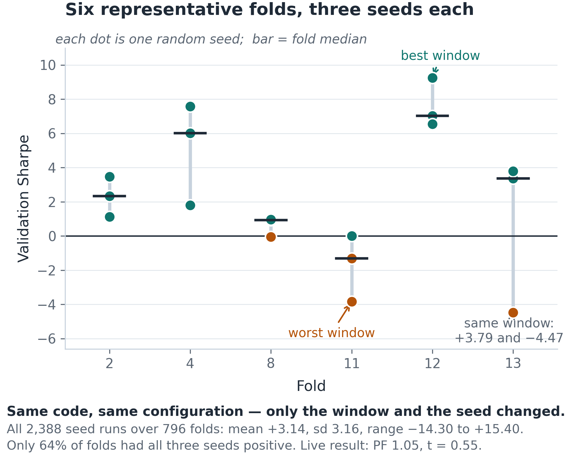
Figure 2. Validation Sharpe by fold and by seed, plotted from the table above. Each dot is one random seed and the horizontal bar is the fold median. Fold 11 and fold 12 differ only in the historical window; the two outer seeds of fold 13 differ only in initialization. The 2,388 seed evaluations recorded across the project average +3.14 with a standard deviation of 3.16.
The spread of results is large. Fold 12 had a median Sharpe of 7.02 while fold 11 had -1.31 with the same code and configuration; only the historical window changed. Even inside fold 13, one seed returned +3.79 and another -4.47. Across the project I logged 796 completed folds and 2,388 individual seed evaluations. Mean seed Sharpe was +3.14, standard deviation was 3.16, the range was -14.30 to +15.40, and only 64% of folds had all three seeds positive.
This is why the live result matters so much. Validation Sharpe averaged above 3, but the demo ended at profit factor 1.05 with t = 0.55. If I had trained once on one fold and one seed, it would have been very easy to select a result that looked impressive and was not representative.
5.5 Multi-Seed Robustness and Promotion Gates
If a model only works for some random seeds, I consider it lucky rather than robust.
def multi_seed_evaluation(model_fn, train_df, val_df, config, n_seeds=3, seed_base=0):
    results = []
    for i in range(n_seeds):
        seed = seed_base + i * 1000
        model, vec = model_fn(train_df, config, seed=seed)
        metrics = evaluate_model(model, vec, TradingEnv(val_df, config))
        metrics["seed"] = seed
        results.append(metrics)
        print(f"Seed {seed}: Sharpe={metrics['sharpe_ratio']:.3f} "
              f"PF={metrics['profit_factor']:.2f} trades={metrics['n_trades']:.0f}")

    sharpes = np.array([r["sharpe_ratio"] for r in results])
    return {
        "mean_sharpe": float(sharpes.mean()),
        "std_sharpe": float(sharpes.std()),
        "min_sharpe": float(sharpes.min()),
        # Stability as a dispersion penalty, not a min/max ratio: the ratio is
        # undefined or misleading when the maximum is near zero or negative.
        "stability": float(1.0 / (1.0 + sharpes.std())),
        "all_positive": bool((sharpes > 0).all()),
        "worst_pf": float(min(r["profit_factor"] for r in results)),
        "seed_results": results,
    }


def sanity_check(metrics: Dict, config: Dict) -> Tuple[bool, list]:
    failures = []
    if metrics.get("insufficient_data"):
        failures.append("insufficient trades or bars to evaluate")
    if metrics.get("expectancy", -1) <= 0:
        failures.append(f"non-positive expectancy: {metrics.get('expectancy'):.6f}")
    if metrics.get("profit_factor", 0) < config.get("MIN_PROFIT_FACTOR", 1.05):
        failures.append(f"PF {metrics.get('profit_factor'):.2f} below minimum")
    if metrics.get("n_trades", 0) < config.get("MIN_TRADES", 30):
        failures.append(f"only {metrics.get('n_trades'):.0f} trades")
    if metrics.get("max_drawdown", 1.0) > config.get("MAX_DRAWDOWN_LIMIT", 0.30):
        failures.append(f"max DD {metrics.get('max_drawdown'):.2%} too large")
    ev = metrics.get("explained_variance", np.nan)
    if np.isfinite(ev) and ev < config.get("MIN_EXPLAINED_VARIANCE", 0.05):
        failures.append(f"explained variance {ev:.4f} too low")
    return len(failures) == 0, failures
5.6 A Warning About Repeated Testing
Multi-seed tests and promotion gates reduce noise for one candidate. They do not solve the problem created by testing many different candidates against the same final window.
Over about two months I ran roughly 1,100 hyperparameter trials against the same final test window, and only one model was promoted. With that many attempts, the best result will partly reflect the specific behavior of that window. This multiple-testing effect is a reasonable explanation for why the system could show walk-forward Sharpe near 5 and later produce a live profit factor of 1.05 with t = 0.55.
There are several ways to reduce this: move the final test window forward instead of querying the same one forever, use a deflated-Sharpe type correction that considers the number of trials, and treat the live demo as the real out-of-sample test.
5.7 Hyperparameter Search with Optuna
I use Optuna for the hyperparameter search. Each trial trains several seeds, and I prune the trial as soon as one seed fails the sanity checks. The mistake was in my scoring function, not in Optuna. My first score combined reward-based Sharpe, reward-based Sortino and a min/max consistency ratio across seeds. In other words, I was optimizing statistics of the shaped reward, and then averaging in a way that could hide the worst seed.
def compute_composite_score(results: Dict) -> float:
    """Single objective built from EQUITY-based metrics only.

    Deliberately includes what the original version omitted: drawdown,
    turnover, and tail behavior across seeds. A candidate cannot buy a
    high score with one lucky seed - the worst seed carries real weight.
    """
    seeds = results["seed_results"]
    mean_pf = float(np.mean([r["profit_factor"] for r in seeds]))
    worst_pf = float(min(r["profit_factor"] for r in seeds))
    worst_dd = float(max(r["max_drawdown"] for r in seeds))
    mean_calmar = float(np.mean([r["calmar_ratio"] for r in seeds]))
    turnover = float(np.mean([r["turnover"] for r in seeds]))

    pf_score = np.clip((mean_pf - 1.0) / 0.5, 0.0, 1.0)        # PF 1.5 = full marks
    tail_score = np.clip((worst_pf - 1.0) / 0.3, 0.0, 1.0)     # worst seed must profit too
    calmar_score = np.clip(mean_calmar / 3.0, 0.0, 1.0)
    dd_score = np.clip(1.0 - worst_dd / 0.25, 0.0, 1.0)        # 25% DD = zero marks
    stability = results["stability"]                            # dispersion penalty
    churn_penalty = np.clip(turnover / 0.05, 0.0, 1.0) * 0.10   # discourage overtrading

    score = (
        0.30 * pf_score
        + 0.25 * tail_score
        + 0.15 * calmar_score
        + 0.20 * dd_score
        + 0.10 * stability
        - churn_penalty
    )
    return float(np.clip(score, 0.0, 1.0))
The search setup itself is normal: TPE sampling, median pruning and a persistent study so an interrupted run can continue. I start a new study when I change something that changes the reward landscape, because old trials then describe a different problem. The caveat from section 8.1 still applies: a good optimizer searches efficiently, but that also makes it easier to overfit the search process to a test window, so the multiple-testing correction becomes more important.
6. Deployment Safeguards: Contract, Normalization, Risk Controls
For me, the biggest production risk is often not the model quality. It is giving a valid model inputs that are different from the ones used during training. This can be difficult to notice because the process still runs and trades; it just behaves incorrectly.
6.1 The Manifest Contract
Every promoted model therefore includes a machine-readable description of the inputs and settings it expects. The live trader builds the same description from its local configuration and refuses to load the model if they do not match.
import hashlib
import json
from datetime import datetime

from features import FEATURE_COLUMNS


def _hash(obj) -> str:
    return hashlib.sha256(
        json.dumps(obj, sort_keys=True, separators=(",", ":"), default=str).encode()
    ).hexdigest()


def build_contract(config: Dict) -> Dict:
    feature_schema = {
        "symbol": config["SYMBOL"],
        "timeframe_minutes": config["TIMEFRAME_MINUTES"],
        "lookback_bars": config["LOOKBACK_BARS"],
        "feature_columns": FEATURE_COLUMNS,
        "obs_dim": config["LOOKBACK_BARS"] * len(FEATURE_COLUMNS) + 5,
        "max_position_bars": config["MAX_POSITION_BARS"],
    }
    execution_schema = {
        "sl_atr_mult": config["SL_ATR_MULT"],
        "tp_atr_mult": config["TP_ATR_MULT"],
        "risk_pct": config["RISK_PCT"],
    }
    contract = {
        "profile_id": config["DEPLOYMENT_PROFILE_ID"],
        "feature_schema": feature_schema,
        "feature_schema_hash": _hash(feature_schema),
        "execution_schema": execution_schema,
        "execution_schema_hash": _hash(execution_schema),
    }
    contract["contract_hash"] = _hash(
        {k: contract[k] for k in ("feature_schema_hash", "execution_schema_hash")}
    )
    return contract


def validate_contract(manifest: Dict, runtime_config: Dict) -> None:
    """Raise rather than trade on a mismatched model."""
    expected = build_contract(runtime_config)
    got = manifest.get("contract")
    if not got:
        raise RuntimeError("Model has no contract; refusing to load.")
    for key in ("feature_schema_hash", "execution_schema_hash", "contract_hash"):
        if got.get(key) != expected.get(key):
            raise RuntimeError(
                f"CONTRACT MISMATCH on {key}.\n"
                f"  model  : {got.get('feature_schema')}\n"
                f"  trader : {expected.get('feature_schema')}\n"
                "Refusing to trade. Update the trader to match, or do not deploy."
            )
This turns silent mistakes into startup errors: an incorrect observation size, a changed feature list, or a different holding horizon. I also keep promotion as a separate step. Training writes candidate files into an isolated directory, then a reviewable promotion step copies the model, normalization state and manifest into production, updates the manifest paths and keeps a backup of the previous version.
6.2 Warm-Up History in Live Inference
My first EA sent only 20 bars to the feature code, even though the rolling windows used 20, 26, 50 or 100 bars. The longer-window values became NaN and were then silently replaced with zeros. So the live model was receiving feature patterns that were not present during training.
REQUIRED_BARS = MAX_WARMUP_BARS + config["LOOKBACK_BARS"] + 10   # e.g. 120 + 16 + 10


def build_live_observation(raw_bars: list, position_state: Dict, config: Dict) -> np.ndarray:
    if len(raw_bars) < REQUIRED_BARS:
        raise ValueError(f"Need {REQUIRED_BARS} bars for warm-up, received {len(raw_bars)}")

    # Explicit key mapping - never rely on DataFrame column order.
    df = pd.DataFrame(raw_bars).rename(columns={
        "o": "open", "h": "high", "l": "low", "c": "close",
        "v": "tick_volume", "s": "spread", "t": "time",
    })
    df = compute_features(df)                       # the SAME module used in training

    lookback = config["LOOKBACK_BARS"]
    window = df.iloc[-lookback:][FEATURE_COLUMNS]
    if window.isna().any().any():
        raise ValueError("NaNs in live feature window - insufficient warm-up history")

    flat = window.values.flatten().astype(np.float32)

    # Position features must match training EXACTLY, including SL/TP distances.
    price = float(df.iloc[-1]["close"])
    pos = position_state["position"]
    if pos != 0:
        entry = position_state["entry_price"]
        unrealized = pos * (price - entry) / entry
        duration = min(position_state["position_bars"] / config["MAX_POSITION_BARS"], 1.0)
        sl_dist = pos * (price - position_state["stop_loss"]) / price
        tp_dist = pos * (position_state["take_profit"] - price) / price
    else:
        unrealized = duration = sl_dist = tp_dist = 0.0

    pos_features = np.array(
        [float(pos), unrealized * 10, duration, sl_dist * 100, tp_dist * 100],
        dtype=np.float32,
    )
    return np.concatenate([flat, pos_features])
6.3 Position Sizing
My original EA also used a fixed lot size. In practice, this is not a sound position-sizing approach because 0.1 lots represents a different percentage of the account as equity changes, while the money at risk also varies with volatility. I now size the position from the stop distance and a fixed percentage of current equity. I use the broker's own symbol values, such as tick value, tick size and volume step, instead of assuming a gold multiplier because contract specifications differ between brokers.
import math


def position_size(equity: float, entry: float, stop_loss: float,
                  symbol_info, config: Dict) -> float:
    """Lots such that a stop-out costs RISK_PCT of equity.

    Uses broker-reported tick value/size and the volume grid rather than an
    assumed contract multiplier, so the same code is correct across brokers.
    Returns 0.0 when the trade cannot be sized safely - the caller must skip.
    """
    stop_distance = abs(entry - stop_loss)
    if stop_distance <= 0 or symbol_info is None:
        return 0.0

    # Value of a one-price-unit move, for one lot, in account currency.
    if symbol_info.trade_tick_size <= 0:
        return 0.0
    value_per_unit = symbol_info.trade_tick_value / symbol_info.trade_tick_size
    if value_per_unit <= 0:
        return 0.0

    risk_amount = equity * config["RISK_PCT"] / 100.0
    raw_lots = risk_amount / (stop_distance * value_per_unit)

    # Snap DOWN to the broker's volume grid, then clamp to its limits.
    step = symbol_info.volume_step
    lots = math.floor(raw_lots / step) * step
    lots = max(symbol_info.volume_min, min(symbol_info.volume_max, lots))

    # Never let rounding push risk above the intended fraction.
    if lots * stop_distance * value_per_unit > risk_amount * 1.5:
        return 0.0
    return round(lots, 2)
6.4 Account-Level Risk Control
A stop on each trade is not enough for account risk. I also want a maximum daily loss, and that state has to survive a process or terminal restart.
def check_kill_switch(config: Dict) -> Tuple[bool, str]:
    """Stateless: recomputed from broker deal history, so a restart cannot reset it."""
    account = mt5.account_info()
    if account is None:
        return False, ""
    day_start = datetime.utcnow().replace(hour=0, minute=0, second=0, microsecond=0)
    deals = mt5.history_deals_get(day_start, datetime.utcnow() + timedelta(minutes=5))
    if deals is None:
        return False, ""

    closes = sorted(
        [d for d in deals if d.magic == config["MAGIC"] and d.entry == mt5.DEAL_ENTRY_OUT],
        key=lambda d: d.time,
    )
    day_pnl = sum((d.profit or 0) + (d.swap or 0) + (d.commission or 0) for d in closes)

    streak = 0
    for d in reversed(closes):
        if (d.profit or 0) + (d.swap or 0) < 0:
            streak += 1
        else:
            break

    limit = -abs(config["DAILY_LOSS_LIMIT_PCT"]) / 100.0 * account.balance
    if day_pnl <= limit:
        return True, f"daily loss {day_pnl:+.2f} breached limit {limit:+.2f}"
    if streak >= config["MAX_CONSECUTIVE_LOSSES"]:
        return True, f"{streak} consecutive losing trades"
    return False, ""
When the daily limit is hit, I block new entries only. Open positions are still managed by their broker-side stops.
6.5 If You Use an MQL5 EA
These are some areas where my first EA implementation needed work:
- Create indicator handles once in OnInit(), not on every call.
- Validate volume against SYMBOL_VOLUME_MIN, SYMBOL_VOLUME_STEP, SYMBOL_VOLUME_MAX.
- Respect SYMBOL_TRADE_STOPS_LEVEL and SYMBOL_TRADE_FREEZE_LEVEL before submitting SL/TP; a stop closer than the broker's minimum is rejected (retcode 10016).
- Measure drawdown on equity, not balance—balance ignores open positions.
- Handle retcodes explicitly: requote, market closed (10018—defer rather than retry-spam), invalid stops, no money.
- Check filling mode support; ORDER_FILLING_IOC is not universal.
- Persist the last processed bar time and the daily trade counter so a restart cannot re-trade a bar already acted on.
- Protocol hygiene if using sockets: length-prefixed framing, request IDs, reconnect with backoff, partial-read handling, and a defined timeout fallback (hold, never guess).
7. What Happened in the Live Demo
This is the section I would most want to read in someone else's article, so here is mine.
The pipeline worked. The alpha did not.
The validation process rejected most candidates, and the champions only improved a little over time. Looking back, this was the system honestly reporting that it had nothing to find.
7.1 Live Demo Results from Broker History
I did not use the model's own accounting to judge the live result. The numbers below come from the broker's closed-deal history, filtered by the magic number. The model and trading loop do not provide any of the performance values. The calculation script is short enough to include in full and can also be run on another account.
"""
reconcile.py - evaluate a live or demo EA from BROKER records only.

Reads closed deals from the MT5 terminal, filters by magic number, and reports
the statistics that actually determine whether a result means anything:
profit factor, expectancy, drawdown, worst losing run, and - most importantly -
the t-statistic, which tells you whether the profit is distinguishable from
zero at all.

    python reconcile.py --magic 123456 --days 180
"""
import argparse
from datetime import datetime, timedelta

import numpy as np
import MetaTrader5 as mt5


def load_closed_trades(magic: int, days: int) -> np.ndarray:
    """Return per-trade net P&L (profit + swap + commission) from broker history."""
    if not mt5.initialize():
        raise RuntimeError(f"MT5 initialize failed: {mt5.last_error()}")
    end = datetime.now()
    deals = mt5.history_deals_get(end - timedelta(days=days), end)
    if deals is None:
        raise RuntimeError(f"history_deals_get failed: {mt5.last_error()}")

    closes = [d for d in deals
              if d.magic == magic and d.entry == mt5.DEAL_ENTRY_OUT]
    closes.sort(key=lambda d: d.time)
    pnl = np.array([(d.profit or 0.0) + (d.swap or 0.0) + (d.commission or 0.0)
                    for d in closes], dtype=float)
    times = [datetime.fromtimestamp(d.time) for d in closes]
    mt5.shutdown()
    return pnl, times


def report(pnl: np.ndarray, times) -> None:
    n = len(pnl)
    if n < 2:
        print("Not enough closed trades to evaluate.")
        return

    wins, losses = pnl[pnl > 0], pnl[pnl < 0]
    gross_profit, gross_loss = wins.sum(), -losses.sum()
    expectancy = pnl.mean()
    sd = pnl.std(ddof=1)

    # Significance: is the mean trade distinguishable from zero?
    t_stat = expectancy / (sd / np.sqrt(n)) if sd > 0 else 0.0
    ci_half = 1.96 * sd * np.sqrt(n)          # 95% CI on CUMULATIVE profit

    # Drawdown on the closed-trade equity curve
    equity = np.cumsum(pnl)
    peak = np.maximum.accumulate(np.concatenate([[0.0], equity]))[1:]
    max_dd = float((peak - equity).max())

    worst_streak = streak = 0
    for x in pnl:
        streak = streak + 1 if x < 0 else 0
        worst_streak = max(worst_streak, streak)

    print(f"Closed trades          : {n}")
    print(f"Net P&L                : {pnl.sum():+,.2f}")
    print(f"Profit factor          : {gross_profit / gross_loss:.2f}"
          if gross_loss > 0 else "Profit factor          : inf")
    print(f"Win rate               : {len(wins) / n * 100:.1f}%  "
          f"({len(wins)} W / {len(losses)} L)")
    print(f"Expectancy per trade   : {expectancy:+,.2f}")
    print(f"Payoff ratio           : {wins.mean() / -losses.mean():.2f}"
          if len(losses) else "Payoff ratio           : n/a")
    print(f"Max drawdown           : {max_dd:,.2f}")
    print(f"Worst losing run       : {worst_streak} consecutive")
    print(f"Per-trade st. dev.     : {sd:,.2f}")
    print(f"t-statistic            : {t_stat:.2f}   "
          f"({'SIGNIFICANT' if abs(t_stat) >= 2 else 'NOT significant'})")
    print(f"95% CI on cumulative   : {pnl.sum():+,.0f} +/- {ci_half:,.0f}")

    # Monthly breakdown - exposes results carried by a single lucky month
    print("\nBy month:")
    months = {}
    for t, x in zip(times, pnl):
        key = t.strftime("%Y-%m")
        months.setdefault(key, []).append(x)
    for key in sorted(months):
        vals = np.array(months[key])
        print(f"  {key}: {len(vals):4d} trades  {vals.sum():+10,.2f}")


if __name__ == "__main__":
    ap = argparse.ArgumentParser()
    ap.add_argument("--magic", type=int, required=True)
    ap.add_argument("--days", type=int, default=180)
    a = ap.parse_args()
    pnl, times = load_closed_trades(a.magic, a.days)
    report(pnl, times)
The output of the script for the account subject to live demo trading is as follows:
Closed trades          : 763
Net P&L                : +3,589.38
Profit factor          : 1.05
Win rate               : 45.1%  (344 W / 419 L)
Expectancy per trade   : +4.70
Payoff ratio           : 1.28
Max drawdown           : 4,440.93
Worst losing run       : 9 consecutive
Per-trade st. dev.     : 236.20
t-statistic            : 0.55   (NOT significant)
95% CI on cumulative   : +3,589 +/- 12,780

By month:
  2026-05:   90 trades   -2,794.00
  2026-06:  180 trades   +4,954.08
  2026-07:  260 trades   -1,124.31
  2026-08:  127 trades     +405.71
Two parts of the output are especially important. First, t = 0.55 means the observed profit is not statistically distinguishable from zero. Second, the monthly results show that almost all of the positive result comes from one month.
The script cannot reconstruct slippage by itself because the broker stores the fill price but not the price I requested. To measure slippage I had to log the requested price when sending each order and compare it later with the fill. Once I did that, I found one of the largest real costs in the whole project, discussed in section 7.3.
7.2 One Month Carries Most of the Result
| Month | Trades | Net |
|---|---|---|
| May 2026 | 90 | -$2,794 |
| June 2026 | 180 | +$4,954 |
| July 2026 | 260 | -$1,124 |
| August 2026 | 127 | +$406 |
Three of the four months are flat or negative. If I remove June, the system loses money. The model was unchanged during these months, so the main difference was the market regime. I would not call this a stable edge.
7.3 The Cost of Trading
The broker reconciliation exposed a cost I had not measured before: -$2,370 of exit slippage across 428 exits, or about a 1.7% drag. It was all on exits because entries are market orders. Compared with $3,589 of realized profit, the slippage was roughly two thirds of the final net result. Swap added another $290 of cost.
A backtest that includes spread but ignores this exit slippage would overstate performance enough to change the sign of this system. For future work, fill reconciliation is one of the first live measurements I would add.
7.4 Known Limitations
There are still important limitations in this setup, and they affect how the results should be interpreted.
Simulation: Execution is bar-based rather than tick-based. When SL and TP are both possible inside a bar, the exact order is unknown and I resolve it pessimistically with SL first. Spread is fixed in simulation although live spread changes and often widens at bad times. Commission is constant, and the simulator does not include swaps, market impact, requotes, rejections or latency-related price movement.
Methodology: Reward shaping is still a strong bias, so the agent can learn the reward design instead of a market pattern. Repeatedly checking one final test window can inflate apparent performance. Random episode starts can also overlap, which means the agent may train on the same historical region many times.
Scope: This is one symbol, one timeframe and one broker's data and execution behavior. I have not shown that the same setup generalizes to other instruments. Also, if the EA depends on an external Python service, the complete system cannot be validated inside the MetaTrader 5 Strategy Tester.
8. Lessons Learned and Conclusion
8.1 What Worked
- Walk-forward validation with a properly sized embargo.
- Multi-seed testing, because it removed models that only worked with a fortunate initialization.
- Realistic cost modeling, which prevented strategies that only profit at zero spread.
- A deployment contract, so a training/live mismatch fails before trading instead of staying hidden.
- Broker-based reconciliation, so significance and execution costs are calculated from actual deal records.
8.2 What Didn't Work
- Raw PnL rewards: behavior became erratic and risk was not controlled so well.
- Large networks—they overfit rapidly; smaller ones generalized better.
- Single-seed evaluation—a poor predictor of anything.
- Reward-based metrics—the most misleading mistake in my original work.
- Building the RL system before running a signal baseline: this cost the most time.
8.3 What I Would Do Differently
- Run the Part 0 baseline before anything expensive. It takes minutes to run, hours to iterate on features, not months, and can stop the project early for the right reason.
- Use supervised learning when the main problem is prediction. I would keep RL for genuinely sequential decisions, for example exit management.
- Test different targets instead of assuming that next-direction is the target the data can support.
- Keep the final test set protected from repeated use from the beginning of the project.
- Look at statistical significance as well as total profit. I would treat t < 2 as unproven even if the absolute profit looks attractive.
8.4 Checklist Before Deploying Any ML or RL Trading System
- Run a supervised signal baseline. If AUC is near 0.50, stop.
- Use temporal splits with purge and embargo of at least the label horizon.
- Evaluate on equity and trades, never on shaped rewards.
- Test multiple seeds and require all of them to pass.
- Save the normalization state with the model.
- Enforce a train/live contract that refuses mismatched models.
- Supply full warm-up history in live inference; raise rather than zero-fill.
- Size positions from equity using broker symbol math, and add an account-level kill switch.
- Measure real slippage from broker history, not from your backtest.
- Report the t-statistic beside the profit.
8.5 Conclusion
Good engineering and careful validation are necessary but not sufficient: they cannot create information that is absent from the data. The project taught a simple, operational lesson — run the signal test before you build the RL system — and then structure the pipeline so the live environment cannot silently diverge from training.
What you should take away and be able to reproduce immediately:
- Part 0: run a supervised baseline (purged walk‑forward + triple‑barrier labels, AUC) to test for extractable signal. If AUC ≈ 0.50, stop and rework features/target or move to another instrument.
- If signal exists, validate RL only on equity/trade outcomes with temporal splits, an embargo at least as long as the label/holding horizon, and multi‑seed training with promotion gates that require all seeds to pass.
- Treat normalization state as part of the deployable model, enforce a manifest contract that the live trader checks at startup, and require full warm-up history rather than zero-filling.
- Measure real execution costs and statistical significance from broker records (profit factor, slippage, t‑stat). Report t < 2 as unproven even if absolute profit looks attractive.
This is not a claim of a stable alpha. It is a practical procedure that will save you months of debugging and prevent common sources of self-deception: optimizing noise, reward-hacking, leakage, and train/live mismatches. If you take one thing from this work, take Part 0 — run the baseline before you build.
References
- Schulman, J., et al. "Proximal Policy Optimization Algorithms." arXiv:1707.06347 (2017)
- de Prado, M. L. "Advances in Financial Machine Learning." Wiley (2018) — triple-barrier labeling, purged cross-validation, embargo, deflated Sharpe ratio
- Bailey, D. and de Prado, M. L. "The Deflated Sharpe Ratio." Journal of Portfolio Management (2014)
- Stable Baselines3 Documentation: https://stable-baselines3.readthedocs.io/
- Optuna Documentation: https://optuna.readthedocs.io/
- MQL5 Documentation: https://www.mql5.com/en/docs
Files Attached to the Article
All paths below are relative to the terminal data folder, which opens from File → Open Data Folder in MetaTrader 5. The Python listings are reference implementations of the code printed in the article. A reader starting from nothing should begin with SETUP.md, which covers installation from an empty machine.
Four files are runnable entry points. Together, they cover the full workflow: baseline_check.py tests for directional signal; run_training.py runs the training pipeline end to end; live_trader.py replaces the Expert Advisor; and reconcile.py evaluates an account using broker records. The remaining files are the modules those four import, each complete and readable on its own.| # | File | Location after unpacking | Description |
|---|---|---|---|
| 1 | baseline_check.py | MQL5\Files\RL_MT5\src\ | Section 2. Triple-barrier labels, purged walk-forward cross-validation and AUC on your own data. Run this before building anything: an AUC near 0.50 means there is no signal to learn. |
| 2 | config.py | MQL5\Files\RL_MT5\src\ | Section 4.4. The single configuration dictionary, serialized into the manifest so that a trained model carries the settings it was trained under. |
| 3 | data.py | MQL5\Files\RL_MT5\src\ | Section 4.3. Bar retrieval from the terminal and OHLCV validation. |
| 4 | features.py | MQL5\Files\RL_MT5\src\ | Section 4.5. The single source of truth for feature computation, imported by both the trainer and the live trader so that no second implementation can drift away from the first. |
| 5 | environment.py | MQL5\Files\RL_MT5\src\ | Section 4.6. Gymnasium trading environment modeling stop loss and take profit, spread, slippage and commission. |
| 6 | train_ppo.py | MQL5\Files\RL_MT5\src\ | Section 4.7. PPO training setup, and saving a model together with its VecNormalize statistics rather than the weights alone. |
| 7 | walk_forward.py | MQL5\Files\RL_MT5\src\ | Section 5.1. Temporal train and test splits with an embargo between them. |
| 8 | evaluate.py | MQL5\Files\RL_MT5\src\ | Section 5.2. Performance metrics computed from the equity curve and realized trades, never from shaped rewards. |
| 9 | multi_seed.py | MQL5\Files\RL_MT5\src\ | Section 5.5. Multi-seed evaluation and the promotion gate that a candidate must clear before it is considered at all. |
| 10 | optuna_objective.py | MQL5\Files\RL_MT5\src\ | Section 5.7. Composite search objective built from equity metrics, weighted toward the worst seed rather than the mean. |
| 11 | contract.py | MQL5\Files\RL_MT5\src\ | Section 6.1. The manifest contract, which refuses to load a model whose training configuration does not match the runtime configuration. |
| 12 | live_inference.py | MQL5\Files\RL_MT5\src\ | Section 6.2. Live observation building with enforced warm-up history, so that long-window features are never computed from too few bars. |
| 13 | position_sizing.py | MQL5\Files\RL_MT5\src\ | Section 6.3. Risk per trade derived from account equity using the broker's own symbol arithmetic. |
| 14 | kill_switch.py | MQL5\Files\RL_MT5\src\ | Section 6.4. Stateless daily-loss and losing-streak halt, recomputed from broker history on every call so that a restart cannot reset it. |
| 15 | run_training.py | MQL5\Files\RL_MT5\src\ | Sections 4 and 5. One command for the whole training path: bar retrieval, validation, features, walk-forward split, PPO training across seeds, the promotion gate and the manifest. This is the file that produces the model the trader needs. --quick proves the wiring in about twenty minutes; --relaxed lowers the promotion gate so a first run yields a model rather than the rejection the real thresholds are designed to produce. |
| 16 | live_trader.py | MQL5\Files\RL_MT5\src\ | Section 6. The process that replaces the Expert Advisor. Composes the contract check, the observation builder, position sizing and the kill switch into the Option A trading loop described in section 4.2: it reads bars from the terminal on each bar close, asks the policy for an action, and sends the order. Start it with --dry-run, which logs every decision without sending anything. It refuses to run on a live account. |
| 17 | reconcile.py | MQL5\Files\RL_MT5\src\ | Section 7.1. Runs as-is. Reads closed deals from the terminal, filters by magic number, and computes profit factor, expectancy, drawdown, worst losing run, the confidence interval, the monthly breakdown and the t-statistic. |
| 18 | requirements.txt | MQL5\Files\RL_MT5\ | Pinned library versions. Stable-Baselines3, Gymnasium and NumPy all introduce breaking changes, and a model trained under one combination may not load under another. |
| 19 | README.md | MQL5\Files\RL_MT5\ | Maps every file to the article section it comes from, and states plainly which files run unmodified and which are listings. |
| 20 | SETUP.md | MQL5\Files\RL_MT5\ | Setup from an empty machine. Written for a reader who has not done this before: that the MetaTrader5 package is Windows-only, which Python version to install, enabling algorithmic trading in the terminal, finding your broker's symbol name, the four commands in order with their expected runtimes, and a table of failure messages against their causes. |
| 21 | architecture.txt | MQL5\Files\RL_MT5\docs\ | The system architecture diagram, the walk-forward layout and the train/test split illustration from sections 4.1, 5.1 and 3.4. |
| 22 | reward_hacking_examples.py | MQL5\Files\RL_MT5\docs\ | Section 3.3. Three ways an agent exploits a badly specified reward function. |
| 23 | overfitting_example.txt | MQL5\Files\RL_MT5\docs\ | Section 3.1. The spurious-pattern illustration. |
| 24 | sample_output.txt | MQL5\Files\RL_MT5\docs\ | The output of reconcile.py for the account discussed in section 7.1, so that the printed results can be compared against a reader's own run. |
| 25 | MQL5.zip | Terminal data folder (File → Open Data Folder) | All of the above in a single archive. Unpack it directly into the terminal data folder and every file is placed in its required location: the archive already contains the MQL5\Files\RL_MT5\ path, so no manual copying or folder creation is needed. Then open a command prompt in MQL5\Files\RL_MT5\, run pip install -r requirements.txt, and the two runnable scripts can be started with python src\baseline_check.py and python src\reconcile.py. |
Risk Disclaimer
Trading involves substantial risk of loss. Nothing in this article is investment advice. Past performance—simulated, demo or live—does not indicate future results.
Warning: All rights to these materials are reserved by MetaQuotes Ltd. Copying or reprinting of these materials in whole or in part is prohibited.
This article was written by a user of the site and reflects their personal views. MetaQuotes Ltd is not responsible for the accuracy of the information presented, nor for any consequences resulting from the use of the solutions, strategies or recommendations described.

 Survival Analysis for Trade Exits: A Discrete-Time Competing-Risks Model in MQL5
 Dandelion Optimizer (DO)
 From Basic to Intermediate: Like Bubbles
 Market Simulation: Position View (VII)

- Free trading apps
- Over 8,000 signals for copying
- Economic news for exploring financial markets
You agree to website policy and terms of use