Neural Networks in Trading: Probabilistic Time Series Forecasting (K2VAE)

Introduction

In recent years, time series analysis has made a real breakthrough. Anomaly detection, classification, and missing value imputation are now handled more accurately and quickly. However, for financial markets, probabilistic forecasting is far more important: it is not simply a matter of predicting an asset's price, but of assessing the range of possible scenarios. Such assessments help traders and analysts develop flexible strategies, manage risks, and make informed decisions.

Classical models are excellent at making short-term forecasts. But look a little further ahead, and errors begin to accumulate, volatility amplifies inaccuracies, and computational costs skyrocket. This is especially true in financial markets, where every event — whether a corporate earnings report or a geopolitical surprise — introduces nonlinearity and changes the rules of the game.

As one possible approach to solving this type of problem, a new framework based on two fundamental ideas was proposed in the paper "K²VAE: A Koopman-Kalman Enhanced Variational AutoEncoder for Probabilistic Time Series Forecasting." First, Koopman theory converts nonlinear processes into a linear form. Imagine that you are looking at a stock price chart through special lenses, and it turns into a straight line — this approach makes it easier to understand the dynamics. Second, the classic Kalman filter carefully processes new data, adjusting the forecast every time new information becomes available: an earnings report, a change in interest rates, or an unexpected event.

The authors of the paper combined these ideas into the K²VAE framework — a lightweight and fast system based on a variational autoencoder. First, KoopmanNet imposes a linear structure on historical price data and indicators. Then, KalmanNet, built on Kalman filter methods, refines the estimates of possible movements and their uncertainty step by step. This architecture enables forecasting over both short- and long-term horizons while maintaining high accuracy and stability.

Key advantages of the K²VAE framework:

• model transparency. The linear component gives traders interpretable signals, rather than being a black box;
• forecast flexibility. You can quickly generate scenarios for various assets: currency pairs, indices, and commodities;
• risk management. Adaptive adjustment of the confidence interval helps reduce the risk of large losses in a timely manner.

As a result, K²VAE becomes a versatile solution for both short-term and long-term forecasts, allowing users to go beyond a single scenario and immediately assess the full range of possible market movements. This significantly improves the effectiveness of portfolio management and the reliability of automated trading strategies — you see not just a point forecast, but a picture of potential risks and opportunities.

The K²VAE Algorithm

In the dynamics of financial markets, we often encounter what appears to be chaos — price fluctuations, sudden spikes in volatility, and the impact of news reports. Koopman theory offers a view from within: instead of trying to tame nonlinearity directly, we transform our system into a special observable space. Here, each state vector xₖ (for example, a basket of quotes or a set of economic indicators) is transformed via the function ψ into a certain observable, where the evolution is described by a linear operator 𝒦. Simply put, we linearize a complex price chart so that it lies along a straight line, which makes it much easier to analyze and forecast the underlying dynamics of the time series. This approach helps distinguish the long-term trend from short-term noise.

However, even with a linear representation, we remain subject to uncertainty: prices change every second, new economic reports are released, and central banks adjust interest rates. This is where the Kalman filter comes into play. This algorithm operates on a simple yet powerful Forecast–Correction principle: first, we predict the current state of the system and estimate our confidence in the prediction (matrix Pₖ), and then, upon receiving the actual measurement (price, trading volume, or macroeconomic indicator), we calculate the Kalman gain Kₖ. We use it to adjust the initial forecast to reflect reality and update our estimate of uncertainty. For a trader, this is equivalent to online updating of the model state using fresh data: company reports, changes in liquidity, or sudden geopolitical events are instantly incorporated into the forecast, minimizing the model’s lag behind the live market.

By combining the system’s linear rollout with adaptive filtering, we obtain a robust foundation for probabilistic forecasting. But to avoid being limited to a single scenario, we bring in the power of a variational autoencoder. VAE turns the problem into conditional generation: the input is historical data X (T most recent observations for N assets), and the output is not a single vector of future values, but a distribution of possible trajectories Y. The key point is the latent variable Z, which accounts for hidden market factors: correlations, cycles, and unexpected shocks. Optimization is performed using a lower bound on the log-likelihood. The first component penalizes the model for poor generation, while the second penalizes it for the latent distribution drifting into extreme regions far from our prior expectations.

In the K²VAE framework, these three components (KoopmanNet, KalmanNet, and VAE) do not simply coexist; rather, they complement each other seamlessly. Overall, the K²VAE architecture follows a clear multistage pipeline, in which each component is responsible for its own stage in the transformation of the analyzed data into an interpretable dynamical model.

First, the Input Token Embedding module splits the original time series into tokens — small fragments of price history or liquidity metrics. This technique is similar to how an analyst divides a price chart into segments with key support and resistance levels: it makes the data more meaningful.

KoopmanNet then maps these tokens into the so-called observable space. Here, the complex nonlinear behavior of time series (correlations between assets, short-term volatility spikes) is decomposed into simple linear components. Using the training procedure, we identify a linear Koopman operator that, when iterated from the first token, builds a model of the evolution. Of course, there is no ideal observable space that makes the system perfectly linear — hence the bias in the forecasts.

After that, KalmanNet comes into play. Like a Kalman filter, it takes a linear forecast and updates itself using new observations, refining the covariance of the multidimensional state and thereby forming a variational posterior Q(Z|X) with clear semantics. This is critically important in finance: we do not just construct a baseline price trajectory; we immediately assess the range of its possible deviations — from sudden gaps to reversals in response to major news events.

Finally, the decoder performs the inverse observable mapping (ψ⁻¹), returning the resulting samples from latent space to the familiar time-series format. It is also responsible for modeling the final distribution P(Y|Z,X) over the planning horizon. Thus, we obtain a ready-to-use future price scenario — not just one, but many probabilistic trajectories, each with its own risk and confidence estimate.

Ultimately, K²VAE transforms raw financial data into a coherent linear dynamical model with adaptive uncertainty refinement and generation of the full spectrum of possible market movements. It is a powerful tool for portfolio planning, risk assessment, and the creation of reliable algorithmic strategies.

Dividing a time series into patches is much more than just a technical trick. In financial analysis, this is similar to the shift from individual tick quotes to five-minute or half-hour candlesticks, which immediately show both the trend and key spikes in volatility. In the K²VAE framework, data preprocessing is based on a similar idea, but goes beyond the conventional channel-independent architecture, in which each channel is processed separately. Instead, the framework’s authors combine all variables (prices of different assets, trading volumes, and technical indicators) within a single patch, allowing the model to naturally account for the cross-influences among them.

First, the context time series X — a matrix of N variables over T time steps — is divided into several equal, non-overlapping segments of length s. Each of these patches contains data for all N indicators at s time points simultaneously, providing a snapshot of market conditions during that period. Next, we flatten each fragment into a vector of dimension N·s and pass it through a linear projection, which compresses the resulting information into a compact embedding representation of dimension d. Thanks to this operation, the model not only learns to look inside each patch, but also automatically identifies the most significant combinations of variables: whether it is the correlation between technology-sector stocks and semiconductor stocks, or synchronized spikes in trading volumes across different market segments.

This almost explosive transition from disparate channels to multidimensional tokens offers several advantages at once. First, the model instantly detects clustered phenomena, when volatility or price trends affect several assets simultaneously. Second, local noise and random jitter within a single patch are smoothed out, which significantly reduces the number of false signals. Third, thanks to the broader coverage of variables, hidden cycles and long-term patterns become more apparent within each token —patterns that, under a traditional approach, might have gone unnoticed or been distorted when channels were processed independently.

Thus, K²VAE receives as input not a set of individual features, but a comprehensive, analysis-ready snapshot of the market environment for each interval s. This serves as the starting point for the subsequent stages.

In real-world financial time series, we encounter several manifestations of nonlinearity at once: the phases of price cycles can shift relative to one another, statistical characteristics change when important reports are released, and sudden news events disrupt established patterns. To tame this complexity, the authors of the K²VAE framework put on Koopman lenses — that is, they mapped tokens from the realm of chaotic oscillations into a space where their evolution becomes simple and linear.

In practice, it looks like this. First, each smoothed embedding vector of the patch X′ᴾ is passed through a small but powerful MLP that acts as the observable function ψ. Simply put, we distill the complex interrelationships between prices and indicators into a new vector xᴾᵢ*, where the underlying dynamics become more discernible.

By collecting all such vectors, we obtain a matrix X*ᴾ, where each row is already a linearly interpretable projection of a single patch. But simply looking at it is not enough. To understand how the system evolves step by step, we use the eDMD (extended Dynamic Mode Decomposition) method, extracting the previous–next pair from X*ᴾ and computing the operator 𝒦loc, which minimizes the discrepancy between them. It is trained so that the first column of X*ᴾ, when multiplied by 𝒦loc, reproduces the second as accurately as possible, and so on to the end of the time series. This technique makes it possible to derive local transition rules step by step.

Moving from the local to the global level, we add a second, trainable component 𝒦glo. Together, they form the full Koopman operator 𝒦 = 𝒦loc + 𝒦glo. It is precisely this that allows us not only to reconstruct historical patches, but also to look confidently into the future by multiplying the first projection x₁ᴾ* by 𝒦ⁿ, 𝒦ⁿ⁺¹, and so on. In this case, the m = L/s patches in observable space correspond one-to-one to L steps in the original series.

As a result, even the most complex interactions between stock prices, trading volumes, and technical indicators are linearized. K²VAE can quickly and accurately generate forecasts for any horizon — from the next few minutes to months ahead. At the same time, the model remains transparent: we can see both the local transition rules and the global trends, while the linear structure enables traders and risk managers to understand what drives the formation of a given scenario.

After KoopmanNet has linearized the main trends and reconstructed the contextual sequence, small residual errors inevitably remain — the difference between the true projections of the patches and their linear approximation. The authors of the K²VAE framework do not ignore these residuals; on the contrary, they collect them into a unified information stream of residuals that shows where and by how much the linear model fell short.

This matrix-based complaint log captures all kinds of surprises: sudden gaps, sharp volume spikes, or news shocks that have not yet been reflected in the Koopman operator.

Next, a lightweight Transformer integrator takes on the role of a wise advisor: it analyzes all this accumulated nonlinearity and turns it into a series of control inputs U = [u₁, …, uₘ]. Each vector uₖ serves as a signal indicating the direction in which the forecast should be adjusted at step k. Because the Transformer can account for relationships among different time points, the model learns to redistribute error information and correct those errors in the most effective way.

Having obtained the control inputs, we build a classical process model.

Here, A is responsible for the basic step-by-step transition, B for the effect of the control input, and wₖ adds a touch of random noise that reflects unpredictable market factors. We take the initial state z₀ from the last ground-truth patch so that the model starts from the most accurate point possible.

Next, we examine the resulting forecast through the lens of the observation model.

Here, H maps the internal state into the forecast format, and vₖ adds measurement noise, reflecting the inaccuracies inherent in the linear part of the model. We treat the previously generated KoopmanNet forecast for the horizon as our primary observation.

The traditional Forecast–Correction cycle allows KalmanNet to dynamically balance linear forecasts with error information. First, we obtain a preliminary forecast ẑₖ and a covariance matrix P̂ₖ, which quantifies the model's confidence.

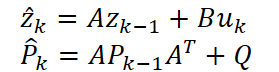
Next, by comparing it with the observation, we calculate the Kalman gain Kₖ. After that, we refine the state and covariance.

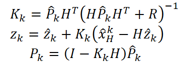
Thus, the model not only refines the forecast but also clearly demonstrates, at every step, how well it understands the market and where it still requires additional confirmation.

To avoid losing the accumulated error information, the framework's authors link the final states to the control inputs via a skip connection.

This ensures that, until KoopmanNet and KalmanNet have mastered all the nuances, the model will make use of all the available information. As training progresses, the magnitude of U tends toward zero — which means that the linear dynamics become increasingly self-sufficient.

As a result, the K²VAE framework produces not just a price forecast, but two related estimates: the value itself and the degree of confidence in it. For traders and risk managers, this is an invaluable two-part signal: the forecast helps plan trades, while the covariance indicates where to proceed with caution and where it may be worth taking a risk. This approach transforms algorithmic trading from a blind pursuit of point predictions into a well-considered risk management strategy.

Finally, we move on to the final stage of generating a probabilistic forecast. At this stage, we already have two key results: the adjusted latent states Z' and the covariance matrices P, which describe our confidence at each stage of the forecast. Together, they define the variational distribution from which we will draw random samples of future scenarios.

To allow gradients to propagate through random sampling, the framework's authors use the familiar reparameterization trick. Instead of directly drawing Z from N(Z',P), they generate standard normal noise ϵ∈N(0,1) and construct:

where L is the lower-triangular matrix from the decomposition P = LLᵀ. Thus, the process itself is differentiable, and gradients flow freely from the loss function to the parameters of both KalmanNet and KoopmanNet.

Next, the authors of K²VAE map the resulting latent vectors Zsample back into the familiar time-series format using a decoder — two symmetric MLPs that mirror the original Koopman-Encoder ψ. The first MLP, which we will denote ψ⁻¹μ, predicts the mean vector μ, while the second, ψ⁻¹σ, predicts the standard-deviation vector σ.

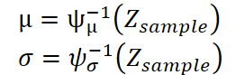
As a result, each generated sample produces a vector of future values along with an estimate of the spread — that is, we immediately see not only the most likely trajectory but also the boundaries of the confidence interval.

To further reinforce the quality of the inverse transformation, the framework authors also pass to ψ⁻¹μ the reconstructed sequence X̂C.

We obtain XRec, which we use to calculate the reconstruction error LRec. This encourages the observable function ψ to construct a truly linear system, and the decoder to accurately map the data back to the original space of prices and indicators.

Finally, after putting everything together, we determine the forecast distribution.

For each sample, the Decoder outputs the vector μ and the vector σ, which are used to construct a full probabilistic forecast: the median, confidence intervals, and extreme scenarios.

In practice, this means that a trader or risk manager immediately gets a comprehensive picture of possible market movements — ranging from a conservative drift within a narrow range to aggressive spikes accompanied by heightened volatility. Thanks to reparameterization and synchronous training of all components (KoopmanNet, KalmanNet, and Decoder), K²VAE provides a smooth, differentiable pipeline where each iteration improves not only the accuracy of the mean forecast but also the reliability of risk estimates.

At the heart of training K²VAE lies a pair of complementary loss functions that together form a powerful mechanism for the model’s self-improvement. The first of these is the classic ELBO objective (Evidence Lower Bound), in which the model aims to achieve two things simultaneously: ensuring that the generated trajectories Y follow the expected distribution, and preventing the latent space Z from straying too far from our prior assumptions.

The first term is a penalty for poor generation of future scenarios: the worse the decoder is at reproducing the distribution of Y from samples of Z, the more it penalizes us. The second term is the KL divergence between our variational posterior Q(Z|X) and a simple standard normal prior P(Z|X)=N(0,I). As a result, we keep the latent space from running away beyond reasonable limits and allow it to smoothly converge to a stable state, where the linear system in the observable space becomes stable.

However, ELBO alone does not guarantee that our observable space will actually behave linearly. This is where the second key component comes into play — reconstruction error.

The framework's authors compare the actual original sequence X with its reconstruction XRec, transformed through the Decoder from the reconstructed Koopman output sequence. The more accurately a model can map data back into the original space, the more accurately and cleanly it builds linear dynamics in the observable layer. This loss function acts as a kind of buttress for the model's foundation, preventing the observable function ψ from deviating from linearity.

Ultimately, the overall training objective is simply the sum of these two parts.

ELBO is responsible for proper generation and a well-structured latent space, while the reconstruction error enforces the rigor of the linear approximation and the quality of the inverse transformation. Together, they force K²VAE not only to learn to generate plausible market scenarios, but also to form an easy-to-understand, interpretable linear-dynamic structure that is resilient to volatility spikes and unexpected market surges. This provides traders and risk managers not just with a forecast, but with a comprehensive, transparent, and reliable decision-making tool.

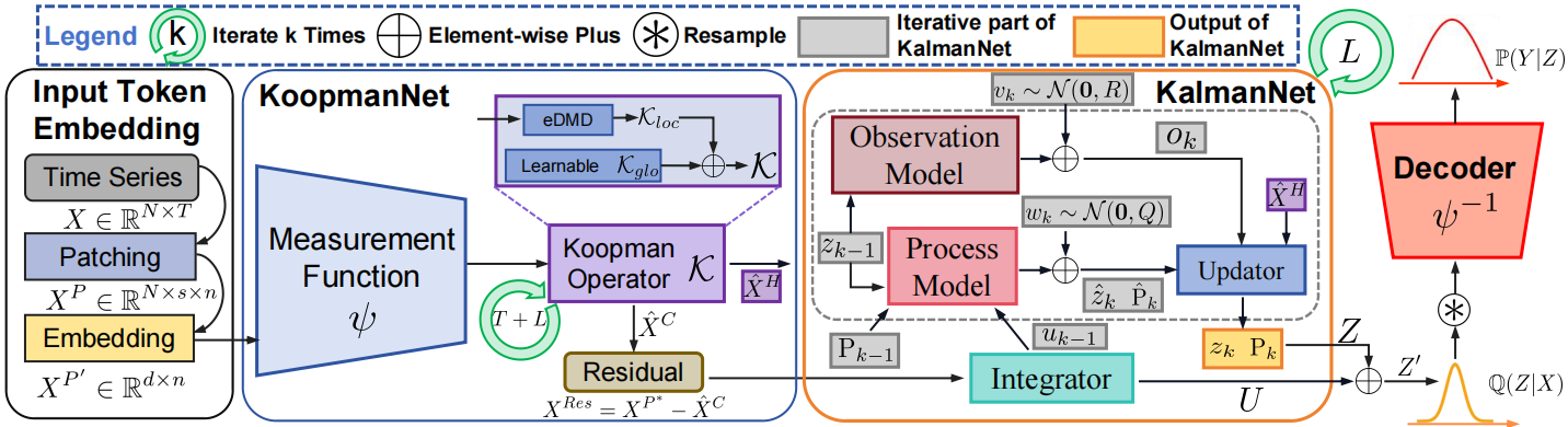
The authors’ visualization of the K²VAE framework is shown below.

Implementation Using MQL5

Now that we have examined all the key components of the K²VAE framework in detail — from the linearization of KoopmanNet dynamics to adaptive uncertainty refinement with KalmanNet and the final VAE decoder — it is time to put theory into practice. In the practical section of our work, we will systematically demonstrate how to implement each of these modules directly within the MQL5 environment: from preparing the source data and generating patches to training the model parameters and producing the final result. This practical guide will help you implement K²VAE step by step in your own algorithmic strategies, while preserving all the flexibility and transparency of the proposed architecture.

As you may have noticed, the core of K²VAE is built around several key matrices — the Koopman operator, the transition and control matrices in KalmanNet, and the weight projections in the encoder and decoder. And unlike the usual Convolution → Activation → Convolution hierarchy in standard neural networks, here the same parameters are involved in several different stages of the pipeline at once. If we were to simply copy this idea as is, we would have to declare separate MLP layers for each step and, consequently, duplicate the weights, which would not only slow down execution and complicate the code, but also distort the concept of a single linear operator.

Therefore, we need to find an alternative solution that will allow us to preserve the concept of shared parameters while integrating them into the existing training mechanism. Here, it is worth recalling an old, tried-and-true approach that we have already used in other projects when we needed trainable matrices outside the standard hierarchy of neural layers.

The idea is to implement a trainable matrix as a two-layer MLP (Multi-Layer Perceptron). The first layer outputs a single fixed value — 1.0 — while the second layer expands it into the entire required parameter matrix. This clever design makes it possible to use standard backpropagation and weight-update mechanisms even for parameters that sit outside the standard structure.

In other words, we are essentially creating a pseudo-layer whose purpose is not to process the input data, but simply to generate a parameter matrix. At first glance, it is computationally useless, but it is precisely through it that the gradient flows, training the second layer — and this is what gives us our matrices A, B, K, H, or, say, ψ.

The advantage of this approach is that it maintains compatibility with the general framework for training neural networks. We do not need to build a separate optimization mechanism or update the weights manually. Everything works according to the standard mechanism: forward pass → error → gradient propagation → parameter update.

Thus, even specialized elements such as Koopman operators or KalmanNet covariance matrices can be integrated into the architecture with full training support.

When a problem requires only a single parameterized matrix, implementing a small MLP within a single object is entirely appropriate. We simply add a couple of internal layers to the structure, feed a constant into the input, and obtain the desired matrix at the output, which we then use in the calculations. It is simple, transparent, and requires no additional architecture.

However, within the KoopmanNet and KalmanNet algorithms, the situation is different: here, we need a whole arsenal of such matrices. Using separate implementations for each one means risking cluttering the architecture and losing readability.

Therefore, we adopted a more versatile and scalable solution — we moved the logic for generating trainable matrices into a separate class, which we will call CParams. This class handles all the work involved in initializing, storing, and updating the weights, as well as returning the desired matrix at the right time. This allows us to:

• centrally manage parameters,
• easily scale the architecture when adding new matrices,
• use a unified generation interface,
• simplify debugging and visualization.

The structure of the new object is shown below and includes a minimal yet functionally complete framework for integration into any neural network architecture.

class CParams  :  public   CNeuronBaseOCL
  {
protected:
   CNeuronBaseOCL    cOne;
   //---
   virtual bool      feedForward(CNeuronBaseOCL *NeuronOCL) override
                        { return FeedForward(); }
   virtual bool      updateInputWeights(CNeuronBaseOCL *NeuronOCL) override
                        { return UpdateInputWeights(); }
   virtual bool      calcInputGradients(CNeuronBaseOCL *NeuronOCL) override  { return true; }
   virtual bool      calcHiddenGradients(CNeuronBaseOCL *NeuronOCL) override { return true; }

public:
                     CParams(void) {};
                    ~CParams(void) {};
   //---
   virtual bool      Init(uint numOutputs, uint myIndex, COpenCLMy *open_cl, uint numNeurons,
                          ENUM_OPTIMIZATION optimization_type, uint batch) override;
   virtual bool      Identity(const int rows, const int cols);
   //---
   virtual bool      FeedForward(void);
   virtual bool      UpdateInputWeights(void);
   //---
   virtual bool      Save(const int file_handle) override;
   virtual bool      Load(const int file_handle) override;
   //---
   virtual int       Type(void) override const  {  return defParams; }
   virtual void      SetOpenCL(COpenCLMy *obj) override;
   //---
   virtual bool      WeightsUpdate(CNeuronBaseOCL *source, float tau) override;
  }; 

A key feature of the implementation is the use of a dummy input, cOne, filled with ones, which is fed to the trainable layer. Thus, the resulting matrix formed at the output becomes the sole object containing the required parameters, ready for direct use.

Under the hood, CParams inherits from the base neural layer CNeuronBaseOCL, which makes it fully compatible with the rest of the framework. The core operating logic resides in the FeedForward and UpdateInputWeights methods, which are implemented by calling the inherited methods of the same names with cOne as the input.

The object is initialized by calling the Init method, which creates the necessary interfaces and configures the connections between components.

bool CParams::Init(uint numOutputs, uint myIndex, COpenCLMy *open_cl, uint numNeurons,
                                      ENUM_OPTIMIZATION optimization_type, uint batch)
  {
   if(!CNeuronBaseOCL::Init(numOutputs, myIndex, open_cl, numNeurons, optimization_type, batch))
      return false;
   if(!cOne.Init(numNeurons, 0, OpenCL, 1, optimization, iBatch))
      return false;
   cOne.SetActivationFunction(None);
   if(!cOne.getOutput().Fill(1))
      return false;
//---
   return true;
  }

A careful implementation allows us to completely hide all the complexities associated with supporting forward and backward passes, parameter optimization, and buffers in an OpenCL context, leaving the user to specify only the matrix shape and purpose declaratively.

The final result is a versatile, scalable, and reusable block of trainable parameters suitable for complex computation graphs. In other words, we get a flexible equivalent of nn.Parameter from PyTorch, but within the MQL5 environment with OpenCL support.

It is worth noting one important detail: forward-pass operations (FeedForward) in the CParams object are performed exclusively during training. This makes sense — after all, it is at this very moment that the weight matrix must be adapted to the model’s errors and adjusted based on backpropagation.

bool CParams::FeedForward(void)
  {
   if(!bTrain)
      return true;
//---
   return CNeuronBaseOCL::feedForward(cOne.AsObject());
  }

However, in production mode — that is, when using a trained model for forecasting or decision-making — there is no need to recalculate the matrix. The matrix produced by training becomes a static parameter — it no longer changes and does not require any additional operations, especially resource-intensive calls to OpenCL kernels.

Thus, when switching to production mode, we essentially lock in the parameters and can safely disable the forward pass, thereby sparing the system from unnecessary computations. This reduces the load on computing resources, speeds up model operation, and improves its stability.

This approach is a classic example of the separation of computational phases, in which training and deployment are strictly distinguished in terms of both logic and workload. This makes the architecture not only more understandable and flexible, but also more predictable during operation, which is especially important in real-time systems.

The complete code for the CParams object and all of its methods is provided in the attachment.

We have already done a tremendous amount of work: we have explored the theoretical foundations of the K²VAE framework, examined its key modules in detail, and even implemented the CParams object — a universal generator of parameterized matrices that is indispensable in the model’s architecture. We now face a more ambitious challenge: to establish clear and consistent logic for the entire framework, where every detail is an essential component of a well-oiled machine.

But there is no need to rush here. Setting up such a system requires a clear mind, attentiveness, and a fresh perspective. That is exactly why we are taking a break until our next article and will return with renewed energy and fresh inspiration.

Conclusion

In this article, we explored K²VAE, a powerful and promising framework that combines the advantages of linear dynamics, variational inference, and adaptive filtering. Its main strength lies in its ability to linearly approximate complex nonlinear processes in a latent observable space, while remaining robust to noise and systematic deviations. This provides not just a model, but a tool with a high degree of interpretability, flexibility, and accuracy — one that is particularly relevant for time series analysis and forecasting market dynamics.

We have only just begun to untangle the web of ideas that underlie the K²VAE framework. In this article, we took the first steps — from the theoretical foundations to the implementation of key components such as parameter matrices and the general-purpose CParams class, which handles all weight management outside the standard neural network architecture. This marked an important step in preparing to construct the model's complete logic.

However, there is much more work ahead. We need to bring together disparate elements into a single, coherent system: implement filtering mechanisms, organize probabilistic dynamics in the latent space, and assemble the Encoder, Integrator, KalmanNet, and Decoder architecture into a single whole. It is no easy task, but it is precisely this that will enable the model to become a truly intelligent decision-making system.

We are not wrapping things up — we have merely outlined the trajectory. The main developments are still to come. So it makes sense to take a short break so we can continue our journey with renewed energy in the next part.

References

• K²VAE: A Koopman-Kalman Enhanced Variational AutoEncoder for Probabilistic Time Series Forecasting
• Other articles in this series

Programs used in this article

#	Name	Type	Description
1	Study.mq5	Expert Advisor	Expert Advisor for offline model training
2	StudyOnline.mq5	Expert Advisor	Expert Advisor for online model training
3	Test.mq5	Expert Advisor	Expert Advisor for model testing
4	Trajectory.mqh	Class library	Structure for describing the system state and model architecture
5	NeuroNet.mqh	Class library	Class library for creating a neural network
6	NeuroNet.cl	Library	Code library for the OpenCL program