Training Neural Networks on Oscillators Without Look-Ahead Bias

Introduction to Look-Ahead Bias, or Why Machine Learning Models Do Not Work on New, Non-Stationary Data

For traders who use machine learning, data preparation is an important part of experiments in developing trading systems. Indicators or price increments are typically fed into the model. Future price increments — that is, how the price chart behaved in the future — are often used as labels.

This method of trade labeling has a particularly problematic feature that leads to poor model performance on new, non-stationary data after training on historical data. The ineffectiveness of this labeling method stems from “look-ahead bias,” which is defined as a model's distortion or bias relative to true patterns. Look-ahead bias in the analysis of financial time series occurs when a model or strategy uses information that was not available at the time the decision was made.

The consequences of this are:

• Inflated and unrealistic results on historical data (backtest). The model demonstrates nearly perfect profitability because it essentially “peeked at the answers” during training.
• A sharp drop in performance on out-of-sample (OOS) data and in live trading. When a model encounters new data where the future is unknown, it cannot identify the ideal patterns to which it has “become accustomed,” and its predictions become useless.
• Low model robustness (stability). The strategy turns out to be overfitted to historical data and unable to adapt to changing market volatility and regimes.

Researchers often underestimate this problem as they search through features that would both match the labels as closely as possible and predict them. However, such a match can never be achieved because of the random and idealized nature of the labels themselves.

There is a need to use a different, more realistic labeling scheme in which information from the future is not available.

Trade Labeling Based on Oscillators to Eliminate Look-Ahead Bias

This article proposes oscillator-based trade labeling methods without look-ahead. They make it possible to create more realistic label sets that are robust to new data and have a low classification error rate. Since oscillators generate buy and sell signals without look-ahead, machine learning algorithms are not exposed to labeling bias and remain effective over the entire historical range for the trading instruments. Because oscillators have a fixed formula and defined overbought and oversold levels, models are trained with low error and perform well in cross-validation, since the task boils down to a simple approximation of the function of a single oscillator or a set of oscillators.

Despite the appeal of this approach, it has a number of drawbacks. First, not every time series can be accurately predicted or labeled using just a single oscillator. Often, overbought and oversold zones are inaccurate and uninformative, leading to false signals and losses. Second, there is the issue of choosing the type, formula, and period of the oscillator, as well as the correct overbought and oversold zones. In addition, it is necessary to test multiple trading instruments to determine which ones oscillators produce the best forecasts on. Third, oscillators are reversal indicators. In trending markets, they do not provide clear predictions about future market dynamics and tend to “get stuck” in extreme positions, so it is better to use them on ranging instruments, where the probability of mean reversion from these zones is relatively high.

Machine Learning as a Tool for Quickly Developing and Refining a Strategy

One could say that the easiest approach would be to select an oscillator tailored to a specific time series, optimize the conditions for opening trades, and test the algorithm's performance using historical data. However, the process of creating such strategies can also be standardized by adding a couple of classifiers that will be responsible for generating trading signals.

The advantage of this approach is that trade labeling based on oscillators is more flexible than relying on strict signals for opening and closing trades. You can add a number of other conditions to the labeling without having to rewrite the entire strategy, while the model training algorithm always remains the same. When trading strategies are hard-coded, the logic of the code becomes exponentially more complex with each new indicator or condition added. But a machine learning algorithm is agnostic to how many features it has to work with: it will automatically assess the importance of each one and make a prediction by weighing all the factors. This makes it easy to run experiments by adding and removing features in bulk and trying different labeling functions without modifying the core of the trading system.

A Library of Oscillators That You Can Extend with Your Own Trade Labelers

I've written several oscillator-based trade labelers. A complete list of labeling functions in the oscillators_labeling.py library.

get_labels_cci(dataset, cci_period=20, oversold_level=-100.0, overbought_level=100.0) -> pd.DataFrame
get_labels_stochastic(dataset, stoch_period=14, smooth_k=3, oversold_level=20.0, overbought_level=80.0) -> pd.DataFrame
get_labels_bb(dataset, bb_period=20, num_std=2.0) -> pd.DataFrame
get_labels_fourier(dataset, lookback_period=20, high_pass_cutoff_idx=5, std_multiplier=1.5) -> pd.DataFrame
get_labels_rsi(dataset, rsi_period=14, oversold_level=30.0, overbought_level=70.0) -> pd.DataFrame
get_labels_profit_rsi_profit_check(dataset, rsi_period=14,
                            oversold_level=30.0, overbought_level=70.0,
                            min_forecast_period=1, max_forecast_period=15,
                            markup=0.0) -> pd.DataFrame

The library includes functions based on well-known indicators such as CCI, Stochastic, Bollinger Bands, and RSI, as well as functions based on Fourier decomposition (for true connoisseurs of finding cyclic components in time series). Special attention will be given to the last experimental RSI-based function: a check for trade profitability has been added to it.

Configuring trade labelers comes down to setting the oscillator periods and the overbought and oversold zones. The conditions for trade labeling are the same for all of them: if the price is above the overbought level, a sell signal is generated, and vice versa. If the price is between the levels, the signal is labeled as “do not trade.”

Since not all trades will be profitable, a function has been added to check their profitability. This trade labeler already introduces look-ahead bias, but it helps make the balance curve smoother.

What Happens Inside Labeling Functions and How to Create Your Own

Let's examine the entire process of trade labeling using the RSI oscillator as an example. Despite the apparent amount of code, there is a simple way to create your own trade labelers using AI. To do this, simply give the AI this example and ask it to do the same thing, but for a different oscillator. So if you're not familiar with Python or some of its features, this is a great option and will save you time.

The first block in calculating labels is a function for building the indicator based on closing prices. It returns the indicator values. Numba is used to speed up calculations. The next function compares the current oscillator values with the threshold values and returns labels. The third function calls the first two, then adds a column with labels to the DataFrame passed to it and returns it. The fourth additional function does the same thing as the third, but with an additional check of whether the trades are profitable. It labels buy and sell trades not only based on threshold conditions, but also checks whether these trades generated a profit; otherwise, they are labeled as "do not trade."

@njit
def calculate_rsi(close_data, period=14):
    """RSI exponential smoothing (Wilder method)"""
    rsi = np.zeros(len(close_data))
    
    # First calculation — simple average
    gains = 0.0
    losses = 0.0
    for j in range(1, period + 1):
        change = close_data[j] - close_data[j - 1]
        if change > 0:
            gains += change
        else:
            losses += abs(change)
    
    avg_gain = gains / period
    avg_loss = losses / period
    
    if avg_loss == 0:
        rsi[period] = 100.0
    else:
        rs = avg_gain / avg_loss
        rsi[period] = 100.0 - (100.0 / (1.0 + rs))
    
    # Exponential smoothing for the remaining values
    for i in range(period + 1, len(close_data)):
        change = close_data[i] - close_data[i - 1]
        gain = max(change, 0.0)
        loss = max(-change, 0.0)
        
        # Wilder's exponential smoothing
        avg_gain = (avg_gain * (period - 1) + gain) / period
        avg_loss = (avg_loss * (period - 1) + loss) / period
        
        if avg_loss == 0:
            rsi[i] = 100.0
        else:
            rs = avg_gain / avg_loss
            rsi[i] = 100.0 - (100.0 / (1.0 + rs))
    
    return rsi

@njit
def calculate_labels_rsi(close_data, rsi_data, 
                         oversold_level=30.0, overbought_level=70.0):
    """
    RSI levels-based labeling.
    """
    labels = []
    
    for i in range(len(close_data)):
        curr_rsi = rsi_data[i]
        
        # Buy signal: RSI in the oversold zone
        if curr_rsi < oversold_level:
            labels.append(0.0)  # Buy
        
        # Sell signal: RSI in the overbought zone
        elif curr_rsi > overbought_level:
            labels.append(1.0)  # Sell
        
        else:
            labels.append(2.0)  # Hold — RSI in the neutral zone
    
    return labels

def get_labels_rsi(dataset, rsi_period=14,
                   oversold_level=30.0, overbought_level=70.0) -> pd.DataFrame:
    dataset = dataset.copy()
    
    close_data = dataset['close'].values
    rsi_data = calculate_rsi(close_data, rsi_period)
    dataset['rsi'] = rsi_data

    labels = calculate_labels_rsi(close_data, rsi_data,
                                  oversold_level, overbought_level)

    # Trim the dataset
    dataset = dataset.iloc[:len(labels)].copy()
    dataset['labels'] = labels
    dataset = dataset.drop(columns=['rsi'])
    
    return dataset.dropna()

def get_labels_profit_rsi_profit_check(dataset, rsi_period=14,
                            oversold_level=30.0, overbought_level=70.0,
                            min_forecast_period=1, max_forecast_period=15,
                            markup=0.0) -> pd.DataFrame:
    
    dataset = dataset.copy()
    close_data = dataset['close'].values
    rsi_data = calculate_rsi(close_data, rsi_period)
    
    # Use NaN for initial filling, since for the last max_forecast_period 
    # elements, the future price cannot be determined.
    labels = [np.nan] * len(close_data) 
    
    # Start iterating from the index after which the RSI has already been calculated
    start_index = rsi_period
    
    # Iterate until the end point that still allows the future price to be determined
    for i in range(start_index, len(close_data) - max_forecast_period):
        
        curr_rsi = rsi_data[i]
        curr_pr = close_data[i]
        
        # 1. First, determine the signal based on RSI
        rsi_signal = 2.0 # Hold by default
        
        # Buy signal: RSI in the oversold zone
        if curr_rsi < oversold_level:
            rsi_signal = 0.0  # Buy
        
        # Sell signal: RSI in the overbought zone
        elif curr_rsi > overbought_level:
            rsi_signal = 1.0  # Sell
        
        # 2. If there is a signal (Buy or Sell), we check its profitability
        if rsi_signal != 2.0:
            
            # Select a random forecast period
            rand_period = random.randint(min_forecast_period, max_forecast_period)
            future_pr = close_data[i + rand_period]
            
            # Profitability check for the Buy signal (0.0)
            if rsi_signal == 0.0:
                # A buy trade is profitable if the future price is greater than the current price plus the markup.
                if (future_pr - markup) > curr_pr:
                    labels[i] = 0.0  # Buy - Profitable
                else:
                    labels[i] = 2.0  # Hold - Not profitable
            
            # Profitability check for the Sell signal (1.0)
            elif rsi_signal == 1.0:
                # A sell trade is profitable if the future price is less than the current price minus the markup.
                if (future_pr + markup) < curr_pr:
                    labels[i] = 1.0  # Sell - Profitable
                else:
                    labels[i] = 2.0  # Hold - Not profitable
        
        else:
            # No RSI signal -> Hold
            labels[i] = 2.0
    
    # Trim the dataset and add labels
    dataset['labels'] = labels
    dataset = dataset.iloc[start_index:].copy()
    
    # Remove NaN values (at the end, where the future price cannot be determined)
    return dataset.dropna()

Which Features Should Be Used to Train Models

An interesting aspect of the proposed approach is that it adheres to the principle of "what goes in is what comes out," analogous to "garbage in, garbage out." But in this case, our data is not garbage; rather, it contains quite clear functional relationships between the indicator values and their thresholds. Therefore, the same oscillators used for labeling can be fed into the models as input features. Any other features, such as increments, are also well suited, since they belong to the same time series, and the machine learning model will automatically adjust its parameters to fit the labeling used. The only difference might be that more additional features would be needed to approximate the oscillator function, which would make the model somewhat more complex, as it would contain more parameters. But this may also produce other interesting effects in terms of model variability, with the models differing in their properties.

I suggest three types of features, which you can expand on yourself. These are features based on differences between the price and moving averages, the RSI indicator, and Wilder's RSI indicator.

def get_features(data: pd.DataFrame) -> pd.DataFrame:
    pFixed = data.copy()
    pFixedC = data.copy()
    count = 0

    for i in hyper_params['periods']:
        pFixed[str(count)] = pFixedC -  pFixedC.rolling(i).mean()
        count += 1

    return pFixed.dropna()

def get_features(data: pd.DataFrame) -> pd.DataFrame:
    pFixed = data.copy()
    count = 0

    for period in hyper_params['periods']:
        delta = data.diff()
        gain = (delta.where(delta > 0, 0)).rolling(window=period).mean()
        loss = (-delta.where(delta < 0, 0)).rolling(window=period).mean()
        rs = gain / loss
        pFixed[str(count)] = 100 - (100 / (1 + rs))
        count += 1
    return pFixed.dropna()

def get_features(data: pd.DataFrame) -> pd.DataFrame:
    pFixed = data.copy()
    count = 0

    for period in hyper_params['periods']:
        delta = data.diff()
        gain = delta.where(delta > 0, 0)
        loss = -delta.where(delta < 0, 0)
        
        avg_gain = gain.ewm(alpha=1/period, adjust=False).mean()
        avg_loss = loss.ewm(alpha=1/period, adjust=False).mean()
        
        rs = avg_gain / avg_loss
        pFixed[str(count)] = 100 - (100 / (1 + rs))
        count += 1

    return pFixed.dropna()

A Quick Look at the Training Results After Labeling Without Look-Ahead (No Look-Ahead)

Now everything is ready to test the proposed approach. For the test, let’s use the AUD/CAD currency pair, which is ranging. Let's configure the algorithm's hyperparameters as follows:

hyper_params = {
    'symbol': 'AUDCAD_H1',
    'export_path': '/Users/Program Files/MetaTrader 5/MQL5/Include/Mean reversion/',
    'model_number': 0,
    'markup': 0.00010,
    'stop_loss':  0.01000,
    'take_profit': 0.01000,
    'periods': [i for i in range(5, 50, 5)],
    'backward': datetime(2015, 1, 1),
    'forward': datetime(2021, 1, 1),
}

Next, we'll train the models using each trade labeler in turn (uncomment the one you need) and test them right away.

options = []
for i in range(1):
    print('Learn ' + str(i) + ' model')
    dataset = get_features(get_prices())
    # dataset = get_labels_cci(dataset, cci_period=50, 
    #                          oversold_level=-130, overbought_level=130)
    # dataset = get_labels_stochastic(dataset, stoch_period=30, smooth_k=15,
    #                                 oversold_level=10, overbought_level=90)
    # dataset = get_labels_bb(dataset, bb_period=25, num_std=2)
    # dataset = get_labels_rsi(dataset, rsi_period=9,
    #                          oversold_level=28, overbought_level=72)
    # dataset = get_labels_fourier(dataset, lookback_period=100, high_pass_cutoff_idx=5,
    #                    std_multiplier=1.5)
    dataset = get_labels_profit_rsi_profit_check(dataset, rsi_period=7,
                            oversold_level=30.0, overbought_level=70.0,
                            min_forecast_period=1, max_forecast_period=5,
                            markup=hyper_params['markup'])
    
    
    dataset['meta_labels'] = (dataset['labels'] != 2.0).astype(float)
    data = dataset[(dataset.index < hyper_params['forward']) & (dataset.index > hyper_params['backward'])].copy()
    options.append(fit_final_models(data))

options.sort(key=lambda x: x[0])
data = get_features(get_prices())
test_model(data, 
        options[-1][1:], 
        hyper_params['stop_loss'], 
        hyper_params['take_profit'],
        hyper_params['forward'],
        hyper_params['backward'],
        hyper_params['markup'],
        plt=True)

Below are the results of applying various trade labelers to the data without optimizing their parameters.

Based on CCI

Based on Stochastic

Based on Bollinger Bands

Based on RSI

Based on Fourier

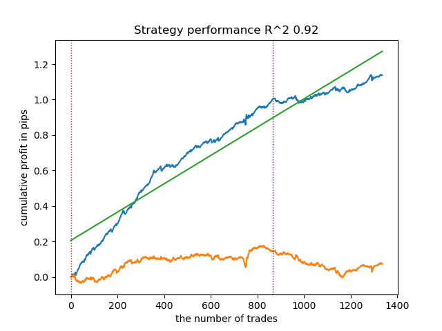
Based on RSI with a profitability check

All the curves, except for the last one, show similar dynamics on the training and test sets. Because the last trade labeler uses look-ahead, its performance on the test set is slightly worse than on the training set. This is due to nothing other than look-ahead, or look-ahead bias. It still allows you to make a profit, since the look-ahead labels are mixed with the original clean labels based on oscillators. The possibilities offered by this approach don't end there, since you can add many different oscillators and even come up with your own.

For comparison, here is an example of a standard trade labeling approach that traders often use and that has appeared in some of my previous articles. This function always looks at future prices to determine the direction of a trade.

def get_labels(dataset, min = 1, max = 15) -> pd.DataFrame:
    labels = []
    for i in range(dataset.shape[0]-max):
        rand = random.randint(min, max)
        curr_pr = dataset['close'].iloc[i]
        future_pr = dataset['close'].iloc[i + rand]

        if (future_pr + hyper_params['markup']) < curr_pr:
            labels.append(1.0)
        elif (future_pr - hyper_params['markup']) > curr_pr:
            labels.append(0.0)
        else:
            labels.append(2.0)
        
    dataset = dataset.iloc[:len(labels)].copy()
    dataset['labels'] = labels
    dataset = dataset.dropna()
    return dataset

It is clear that the model is overfitted, and selecting features tailored to such labels never yields a positive result.

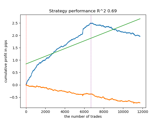
Labeling Based on Look-Ahead

Exporting Trained Models and Facing Real Trading Conditions

Let's train the final model using one of the proposed trade labelers. Let's use RSI-based labeling without look-ahead. To demonstrate the strength of this labeling approach, I trained the model on data from 2015–2017, with 2018–2025 as the forward period.

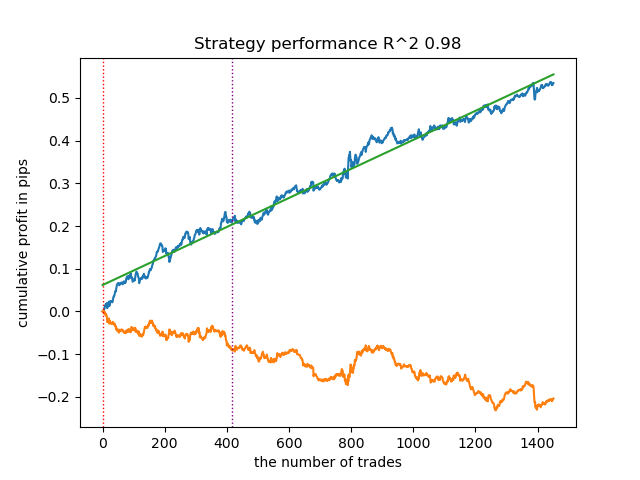
Next, call the function for exporting models in ONNX format to the terminal's Include directory.

export_model_to_ONNX(options[-1],0)

The exported library looks like this:

#include <Math\Stat\Math.mqh>
#resource "catmodel0.onnx" as uchar ExtModel[]
#resource "catmodel_m0.onnx" as uchar ExtModel2[]
int Periods[9] = {5,10,15,20,25,30,35,40,45};

void fill_arays( double &features[]) {
   double pr[], ret[];
   ArrayResize(ret, 1);
   for(int i=ArraySize(Periods)-1; i>=0; i--) {
       CopyClose(NULL,PERIOD_CURRENT,1,Periods[i],pr);
       ret[0] = pr[ArraySize(pr)-1] - MathMean(pr);
       ArrayInsert(features, ret, ArraySize(features), 0, WHOLE_ARRAY); }
   ArraySetAsSeries(features, true);
}

All that's left is to compile the bot and run it in the strategy tester. A distinctive feature of labeling without look-ahead is that the spread is not factored into the labeling at all, which means it can significantly affect the final test results.

Conclusion

Based on a small study, we can conclude that traders often label trades incorrectly for their machine learning models. The article presents trade labeling options that do not lead to model overfitting and consistently perform well over the long term. This opens up new possibilities for analyzing various oscillator-based trade labelers. This approach significantly reduces the number of features and the complexity of the models, which has a positive effect on their robustness, and it completely overturns the conventional paradigm of tailoring features to target labels.

The Python files.zip archive contains the following files for development in a Python environment:

File name	Description
no look ahead.py	Main script for training models
oscillators_labeling.py	Updated module with trade labelers
tester_lib.py	Updated custom strategy tester for machine learning-based strategies
AUDCAD_H1.csv	A file containing quotes exported from the MetaTrader 5 terminal

The MQL5 files.zip archive contains files for the MetaTrader 5 terminal:

File name	Description
no look ahead trader.ex5	The compiled bot from this article
no look ahead trader.mq5	The bot source code from the article
Include//Mean reversion folder	ONNX models and the header file for integrating them with the bot are located here.