

Self Optimizing Expert Advisors in MQL5 (Part 18): Time Lagged Independent Components Analysis
 1 413
1 413
 0
0

In our previous discussion on building self-optimizing expert advisors, we used the moving average indicator as both the signal source for our trading strategy and the target for our statistical model forecasts. This article builds beyond on that exploration by considering how moving average indicators can be augmented with tools from statistical processing to suppress noise in market data. For readers who have not read the previous discussion, a helpful link has been provided here.
Market noise is pervasive and negatively affects our trading strategies. Unfortunately, there are no widely accepted best practices for effectively handling noise. Many solutions have been created over the years by human traders; most notably, a wide array of technical indicators has been developed to alleviate the problem. In this article, we will explore whether these tools may be augmented with statistical signal processing methods. Our proposed solution may allow market technicians to make more effective use of tools they are already familiar with.
It is challenging for practitioners to identify and isolate sources of noise while preserving the true signal in market data. However, if we assume that noise and signal are independent and are mixed in the observed market data, and that their underlying distributions are stable, it may be possible to isolate them. This is the task solved by blind source separation algorithms. Independent Components Analysis (ICA) is the source separation technique we will explore in this discussion.
The ICA algorithm requires the user to specify the number of components that should be identified in the original dataset. The individual components identified by ICA are not explicitly labeled as either noise or true signal. Therefore, we will observe how the accuracy of our model changes as we iteratively increase the number of components to be extracted. Peak performance does not necessarily come from the maximum number of components possible. These unnecessary components could be the channels of noise and other artifacts that were embedded in the original data.
We will apply ICA to market data that has already been filtered by technical indicators. Our market data is filtered by simple moving averages (SMA) and lagged by 5 days. When given time-lagged data, ICA could possibly find independent sources of temporal structure in the data that explain the correlation across time. Additionally, our belief is that, by feeding ICA data that has already been filtered by SMA, we may be able to uncover residual sources of noise that our technical indicators could not filter out.
Getting Started in MQL5
First, we will write a script to fetch the market data we need. We will fetch raw and SMA-filtered data and both corresponding lags to capture as much information as possible. Our script accepts inputs that define the period and smoothing algorithm for the SMA. We set up 4 indicators, one for each price feed, and they all share the same parameters defined by the user. We validate the indicator handlers and attempt to read out their buffers and write them all to file. In total, our dataset has 49 columns.
//+------------------------------------------------------------------+
//|                                                    ICA Filtering |
//|                                      Copyright 2026, CompanyName |
//|                                       http://www.companyname.net |
//+------------------------------------------------------------------+
#property copyright "Copyright 2024, MetaQuotes Ltd."
#property link      "https://www.mql5.com"
#property version   "1.00"
#property script_show_inputs

//+------------------------------------------------------------------+
//| Inputs
//+------------------------------------------------------------------+

input group "File Properties"
input(name="Number of Bars") int size = 10;

input group "Technical Indicators"
input(name="MA Period") int MA_PERIOD = 1;
input(name="MA Type") ENUM_MA_METHOD MA_TYPE = MODE_EMA;

//--- File name
string file_name = Symbol() + " Noise Filter.csv";

//--- Technical indicators
int      ma_h,ma_l,ma_o,ma_c,file_handle;
double   ma_h_reading[],ma_l_reading[],ma_o_reading[],ma_c_reading[];

//+------------------------------------------------------------------+
//| Our script execution                                             |
//+------------------------------------------------------------------+
void OnStart()
  {

//--- Initialize inidcators
   ma_h = iMA(Symbol(),PERIOD_CURRENT,MA_PERIOD,0,MA_TYPE,PRICE_HIGH);
   ma_l = iMA(Symbol(),PERIOD_CURRENT,MA_PERIOD,0,MA_TYPE,PRICE_LOW);
   ma_o = iMA(Symbol(),PERIOD_CURRENT,MA_PERIOD,0,MA_TYPE,PRICE_OPEN);
   ma_c = iMA(Symbol(),PERIOD_CURRENT,MA_PERIOD,0,MA_TYPE,PRICE_CLOSE);

   if(ma_h == INVALID_HANDLE || ma_l == INVALID_HANDLE ||ma_o == INVALID_HANDLE ||ma_c == INVALID_HANDLE)
     {
      //--- We failed to load the indicators
      Comment("Failed To Load Technical Indicators: ",GetLastError());
      return;
     }

   else
     {
      //---Write to file
      file_handle=FileOpen(file_name,FILE_WRITE|FILE_ANSI|FILE_CSV,",");

      for(int i=size;i>=1;i--)
        {

         //--- Update indicator values

         //--- High MA

         if(CopyBuffer(ma_h,0,i,6,ma_h_reading) <= 0)
           {
            Print("An error occurred when copying the High moving average buffer: ",GetLastError());
            return;
           }
         ArraySetAsSeries(ma_h_reading,true);

         //--- Open MA
         if(CopyBuffer(ma_o,0,i,6,ma_o_reading) <= 0)
           {
            Print("An error occurred when copying the Open moving average buffer: ",GetLastError());
            return;
           }
         ArraySetAsSeries(ma_o_reading,true);

         //--- Low MA
         if(CopyBuffer(ma_l,0,i,6,ma_l_reading) <= 0)
           {
            Print("An error occurred when copying the Low moving average buffer: ",GetLastError());
            return;
           }

         ArraySetAsSeries(ma_l_reading,true);

         //--- Close MA
         if(CopyBuffer(ma_c,0,i,6,ma_c_reading) <=0)
           {
            Print("An error occurred when copying the Close moving average buffer: ",GetLastError());
            return;
           }
         ArraySetAsSeries(ma_c_reading,true);

         //--- Fill in the column names
         if(i == size)
           {
            FileWrite(file_handle,
                      //--- Time
                      "Time",
                      //--- OHLC
                      "Open",
                      "High",
                      "Low",
                      "Close",
                      //--- OHLC Lag 1
                      "Open Lag 1",
                      "High Lag 1",
                      "Low Lag 1",
                      "Close Lag 1",
                      //--- OHLC Lag 2
                      "Open Lag 2",
                      "High Lag 2",
                      "Low Lag 2",
                      "Close Lag 2",
                      //--- OHLC Lag 3
                      "Open Lag 3",
                      "High Lag 3",
                      "Low Lag 3",
                      "Close Lag 3",
                      //--- OHLC Lag 4
                      "Open Lag 4",
                      "High Lag 4",
                      "Low Lag 4",
                      "Close Lag 4",
                      //--- OHLC Lag 5
                      "Open Lag 5",
                      "High Lag 5",
                      "Low Lag 5",
                      "Close Lag 5",
                      //--- Indicators
                      "MA O",
                      "MA H",
                      "MA L",
                      "MA C",
                      //--- Indicators lag 1
                      "MA O Lag 1",
                      "MA H Lag 1",
                      "MA L Lag 1",
                      "MA C Lag 1",
                      //--- Indicators lag 2
                      "MA O Lag 2",
                      "MA H Lag 2",
                      "MA L Lag 2",
                      "MA C Lag 2",
                      //--- Indicators lag 3
                      "MA O Lag 3",
                      "MA H Lag 3",
                      "MA L Lag 3",
                      "MA C Lag 3",
                      //--- Indicators lag 4
                      "MA O Lag 4",
                      "MA H Lag 4",
                      "MA L Lag 4",
                      "MA C Lag 4",
                      //--- Indicators lag 5
                      "MA O Lag 5",
                      "MA H Lag 5",
                      "MA L Lag 5",
                      "MA C Lag 5"
                     );
           }

         //--- Fill in the column values
         else
           {
            FileWrite(file_handle,
                      iTime(_Symbol,PERIOD_CURRENT,i),
                      //--- OHLC
                      iOpen(_Symbol,PERIOD_CURRENT,i),
                      iHigh(_Symbol,PERIOD_CURRENT,i),
                      iLow(_Symbol,PERIOD_CURRENT,i),
                      iClose(_Symbol,PERIOD_CURRENT,i),
                      //--- OHLC Lag 1
                      iOpen(_Symbol,PERIOD_CURRENT,i+1),
                      iHigh(_Symbol,PERIOD_CURRENT,i+1),
                      iLow(_Symbol,PERIOD_CURRENT,i+1),
                      iClose(_Symbol,PERIOD_CURRENT,i+1),
                      //--- OHLC Lag 2
                      iOpen(_Symbol,PERIOD_CURRENT,i+2),
                      iHigh(_Symbol,PERIOD_CURRENT,i+2),
                      iLow(_Symbol,PERIOD_CURRENT,i+2),
                      iClose(_Symbol,PERIOD_CURRENT,i+2),
                      //--- OHLC Lag 3
                      iOpen(_Symbol,PERIOD_CURRENT,i+3),
                      iHigh(_Symbol,PERIOD_CURRENT,i+3),
                      iLow(_Symbol,PERIOD_CURRENT,i+3),
                      iClose(_Symbol,PERIOD_CURRENT,i+3),
                      //--- OHLC Lag 4
                      iOpen(_Symbol,PERIOD_CURRENT,i+4),
                      iHigh(_Symbol,PERIOD_CURRENT,i+4),
                      iLow(_Symbol,PERIOD_CURRENT,i+4),
                      iClose(_Symbol,PERIOD_CURRENT,i+4),
                      //--- OHLC Lag 5
                      iOpen(_Symbol,PERIOD_CURRENT,i+5),
                      iHigh(_Symbol,PERIOD_CURRENT,i+5),
                      iLow(_Symbol,PERIOD_CURRENT,i+5),
                      iClose(_Symbol,PERIOD_CURRENT,i+5),
                      //--- Indicators
                      ma_o_reading[0],
                      ma_h_reading[0],
                      ma_l_reading[0],
                      ma_c_reading[0],
                      //--- Indicators lag 1
                      ma_o_reading[1],
                      ma_h_reading[1],
                      ma_l_reading[1],
                      ma_c_reading[1],
                      //--- Indicators lag 2
                      ma_o_reading[2],
                      ma_h_reading[2],
                      ma_l_reading[2],
                      ma_c_reading[2],
                      //--- Indicators lag 3
                      ma_o_reading[3],
                      ma_h_reading[3],
                      ma_l_reading[3],
                      ma_c_reading[3],
                      //--- Indicators lag 4
                      ma_o_reading[4],
                      ma_h_reading[4],
                      ma_l_reading[4],
                      ma_c_reading[4],
                      //--- Indicators lag 5
                      ma_o_reading[5],
                      ma_h_reading[5],
                      ma_l_reading[5],
                      ma_c_reading[5]
                     );
           }
        }

     }
//--- Close the file
   FileClose(file_handle);
  }
//+------------------------------------------------------------------+
Analyzing Our Market Data in Python
Once our dataset has been written out, we load our standard Python libraries to begin analyzing our financial data.
#Import standard Python libraries
import pandas as pd
import numpy as np
import seaborn as sns
import matplotlib.pyplot as plt
Read in the dataset we wrote from the MetaTrader 5 terminal.
#Read in the data
data = pd.read_csv("/ENTER/YOUR/PATH/HERE/EURUSD_Noise_Filter.csv")
data
Let us collect the inputs we have. The first group will be a collection of raw price feeds, the second will contain just their corresponding moving average values, and the final group will be a summation of both.
#Group the inputs
OHLC = data.iloc[:,1:25].columns
MA   = data.iloc[:,25:49].columns
ALL  = data.iloc[:,1:].columns
Now let us define our forecast horizon and forecasting target. Financial time series are unique because we can construct our own targets. Percentage returns, difference from average returns, or just raw returns are a few of the many targets we can choose from. For this discussion, we selected the close moving average itself as a surrogate target to replace the classical target of raw return. The moving average indicator's future values contain traces of preceding values the indicator took. We are motivated to believe that there is some relationship we can learn between the indicator's future value and its lags. We also created binary forms of each target for visualization and analysis.
#Define our forecast horizon
HORIZON = 5

#Label the data with a real valued target
data['C Target']   = data['Close'].shift(-HORIZON) - data['Close'].shift(-1)
data['New Target'] = data['MA C'].shift(-HORIZON) - data['MA C'].shift(-1)

#Label the data with a binary target
data['C Bin Target']   = 0
data['New Bin Target'] = 0

data.loc[data['C Target'] > 0,'C Bin Target'] = 1
data.loc[data['New Target'] > 0,'New Bin Target'] = 1
Drop the final rows that have no label.
#Filter missing rows
data = data.iloc[:-HORIZON,:]
Let us now see how well our surrogate target reflects the underlying target it is intended to represent. We used the binary forms of the targets we created earlier to estimate how often both targets moved in the same direction. We observed that about 81% of the time both targets rose and fell in harmony. Our dataset contained about 7 years of data.
#Correlation between classical target and new target
data.loc[data['C Bin Target'] == data['New Bin Target']].shape[0] / data.shape[0]
0.8126459793126459
This relationship can be observed visually too. In Figure 1 below, we have drawn a vertical black line on the value of 0 along the x-axis. If smoothed returns perfectly matched true returns, there would be no observations left of the black line. Those points indicate positive smoothed returns with negative true returns. We estimated that this is the case about 19% of the time.
#Let us see how well the new target captures the true movement in price
plt.hist(data.loc[(data['New Bin Target'] == 1),'C Target'],bins=100,color='orange')
plt.axvline(0,color='black')
plt.xlabel('True Return')
plt.ylabel('Observed Frequency')
plt.title('Correlation Between Surrogate & Real EURUSD Target')
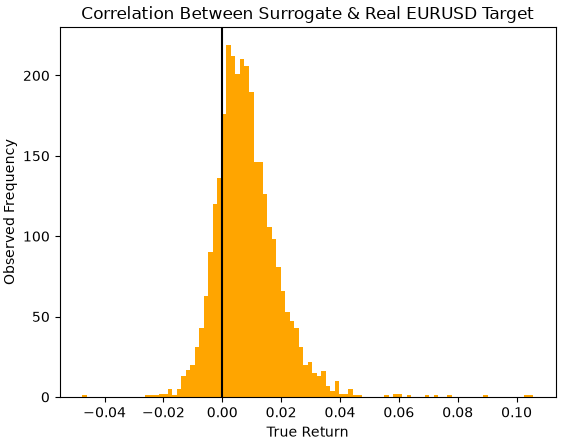
Figure 1: Our surrogate and true targets have a relationship that is not perfect but hopefully reliable.
Import the machine learning libraries we need to start our analysis.
#Comparing our accuracy across targets
from sklearn.linear_model import LogisticRegression as LR
from sklearn.svm import LinearSVC as LSVC
from sklearn.discriminant_analysis import LinearDiscriminantAnalysis as LDA
from sklearn.model_selection import cross_val_score,TimeSeriesSplit
The time series split object helps us to cross-validate our models in a manner that conforms with the goals of time series modeling. The class does not shuffle time series training data during cross-validation; this is an important feature we rely on.
#Setup the time series split object
tscv = TimeSeriesSplit(n_splits=5,gap=HORIZON)
In the for-loop below, we recorded our model's accuracy classifying raw returns as we iteratively increased the number of lags the model is trained on. The results we obtained suggested to us that no significant improvements were made by increasing the number of lags. These results have been visualized as a box plot in Figure 2 below. The middle line in each box plot represents the average cross-validated score we obtained with varying amounts of lag. The midpoints across all bars in the plot appear not too far apart, suggesting that performance is not being improved by lag.
#Record our accuracy on the classical target
classical_scores = []
model = LDA()

for i in np.arange(6):
    classical_scores.append(cross_val_score(model,data.loc[:,OHLC[0:4 + (4*i)]],data['C Bin Target'],cv=tscv,n_jobs=-1,scoring='accuracy'))

sns.boxplot(classical_scores,palette='flare')
plt.title('Modelling The Classical Target With Increasing Lags')
plt.ylabel('Cross-Validation Accuracy out of 100%')
plt.xticks([0,1,2,3,4,5],['No Lags','1 Lag','2 Lags','3 Lags','4 Lags','5 Lags'])
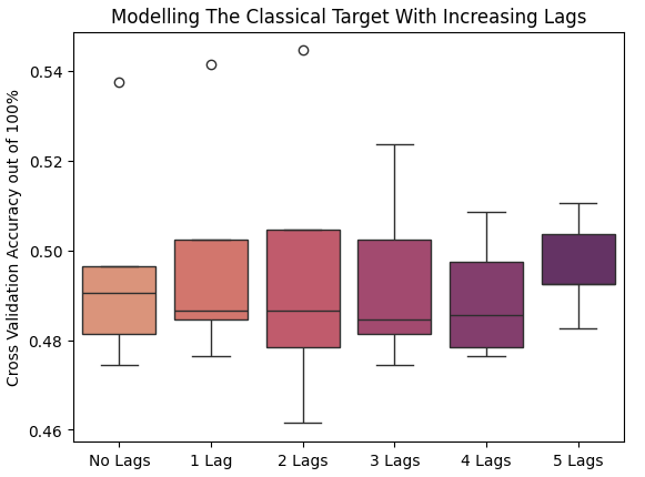
Figure 2: Visualizing the relationship between the raw market returns and the amount of lag used to forecast returns.
Let us repeat the same exercise, but this time we will forecast the change in the moving average indicator as we increase the number of lags. The input data and model type have been preserved across both tests to aim for fair comparison. It appears the data suggests there is a positive relationship between the two. We can observe the mid band of each box plot rising higher and higher as we increased the number of lags the model was trained on.
#Record our accuracy on the new target
new_scores = []
model = LDA()

for i in np.arange(6):
    new_scores.append(cross_val_score(model,data.loc[:,OHLC[0:4+(4*i)]],data['New Bin Target'],cv=tscv,n_jobs=-1,scoring='accuracy'))

sns.boxplot(new_scores,palette='flare')
plt.title('Modelling The New Target With Increasing Lags')
plt.ylabel('Cross-Validation Accuracy out of 100%')
plt.xticks([0,1,2,3,4,5],['No Lags','1 Lag','2 Lags','3 Lags','4 Lags','5 Lags'])
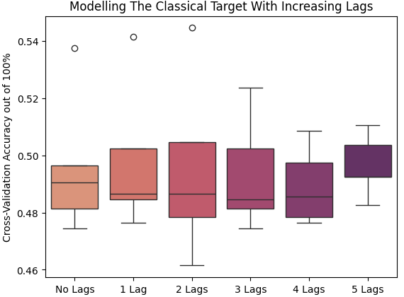
Figure 3: Increasing the number of lags available appears to improve our accuracy at forecasting changes in the SMA indicator.
To visualize the trend, we averaged the score for each target across cross-validation folds and plotted both series side by side. The classical score, depicted by the blue line, sank below the 50% level, denoted by the dashed red line, across all 5 folds. The 50% level marks the best you can get from chance; falling beneath this line may imply the model has no true skill in forecasting the target. Our performance on the new target is captured by the solid red line on the graph. We can observe a positive trend in the surrogate target as we increase the number of lags.
avg_classical_scores = []
avg_new_scores = []

for i in np.arange(len(classical_scores)):
    avg_classical_scores.append(np.mean(classical_scores[i]))
    avg_new_scores.append(np.mean(new_scores[i]))

plt.plot(avg_classical_scores,color='blue')
plt.plot(avg_new_scores,color='red')
plt.axhline(0.5,color='red',linestyle=':')
plt.grid()
plt.ylabel('Cross-Validated Accuracy out of 100%')
plt.title('Comparing Our Average Performance on Both Targets')
plt.xlabel('Cross-Validation Partition')
plt.legend(['Classical Target','New Target'])
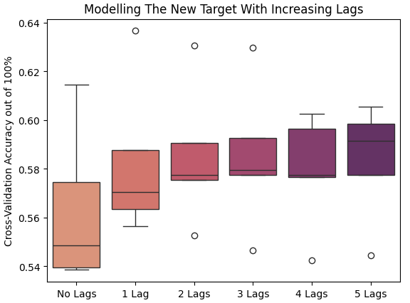
Figure 4: Our average accuracy as we increase the number of lags we use for training the model.
Next, we compare which input group yields the best performance for the easier target. In Figure 5 below, we observe that using raw OHLC data appears to be the worst choice we can make from the data we have. The box plot produced by the raw market returns is wide, suggesting the accuracy of the models varies a lot when given these inputs, which we fear are noisy. The box plot produced by using the filtered indicator data appears tight and reliable, and it produced the highest average performance.
#Record our accuracy on the new target
group_scores = []
model = LDA()

group_scores.append(cross_val_score(model,data.loc[:,OHLC],data['New Bin Target'],cv=tscv,n_jobs=-1,scoring='accuracy'))
group_scores.append(cross_val_score(model,data.loc[:,MA],data['New Bin Target'],cv=tscv,n_jobs=-1,scoring='accuracy'))
group_scores.append(cross_val_score(model,data.loc[:,ALL],data['New Bin Target'],cv=tscv,n_jobs=-1,scoring='accuracy'))

sns.boxplot(group_scores,palette='flare')
plt.title('Modelling The New Target With Different Input Groups')
plt.ylabel('Cross-Validation Accuracy out of 100%')
plt.xticks([0,1,2],['OHLC','Moving Averages','All'])
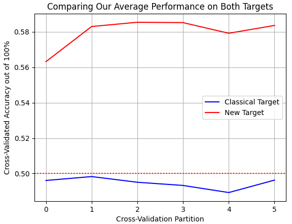
Figure 5: Assessing which group of inputs yields the best performance when forecasting the future SMA indicator value.
Blind Source Separation
We need our blind source separation algorithm. The scikit-learn implementation of FastICA is our algorithm of choice. It handles large datasets well and provides tunable parameters for further enhancing performance.
#Unsupervised learning algorithms
from sklearn.decomposition import FastICA
Let us partition our dataset into its training and test sets.
#Train test split
train = data.iloc[:(-365*4 )-HORIZON,:]
test = data.iloc[:(-365*4 )-HORIZON,:]
We will record how our performance on the task changes as we increase the number of components our ICA algorithm should identify from the smoothed indicator data we feed it. The first recording we will store will be our benchmark performance level when we use the filtered market data as it is. Then, we will set the benchmark score as the best score to be beaten. We quickly outperformed this benchmark and found maximum performance at 18 components. The reader should understand that the initial input data had 24 columns of moving average values and lags. These 24 columns have been projected down to 18.
COMPONENTS = len(MA)-2

model = LSVC()

ica_performance = []
avg_performance = []
train_manifold = 0


ica_performance.append(cross_val_score(model,train.loc[:,MA],train['New Bin Target'],cv=tscv,scoring='accuracy'))
best_score = np.mean(ica_performance[0])
best_components = 0

print(f'Benchmark: {np.mean(ica_performance[0])}')

for i in np.arange(COMPONENTS):

    ica_transformer = FastICA(n_components=(i+1))
    train_manifold = ica_transformer.fit_transform(train.loc[:,MA])
    ica_performance.append(cross_val_score(model,train_manifold,train['New Bin Target'],cv=tscv,scoring='accuracy'))
    #User feedback
    print(f'Number of Components: {i+1} | Performance: {np.mean(ica_performance[i+1])}')
    avg_performance.append(np.mean(ica_performance[i]))
    if(best_score < np.mean(ica_performance[i])):
        best_score = np.mean(ica_performance[i])
        best_components = i+1
        print(f'Improvements Found: Best Score{best_score} | Number of components: {best_components}')
Benchmark: 0.5325648414985591
Improvements Found: Best Score0.5412103746397694 | Number of components: 3
Improvements Found: Best Score0.560806916426513 | Number of components: 5
When we take a closer look at the results we have obtained, we can observe that our performance grows past the original possibilities as we increase the number of lags. It appears the ICA algorithm is exposing meaningful structure in the high-dimensional moving average lags that we were not aware of. This may be helping us separate noise in the data from the signal. However, this is not unlimited growth; our performance appears to plateau after 13 components. For this reason, we chose the second-best option, which was 12 components.
sns.boxplot(ica_performance,palette='flare')
plt.ylabel('Cross-Validated Accuracy out of 100%')
plt.xlabel('Number of ICA Components Used | 0 is the Original Data')
plt.title('Model Accuracy Improves With The Number of ICA Components') 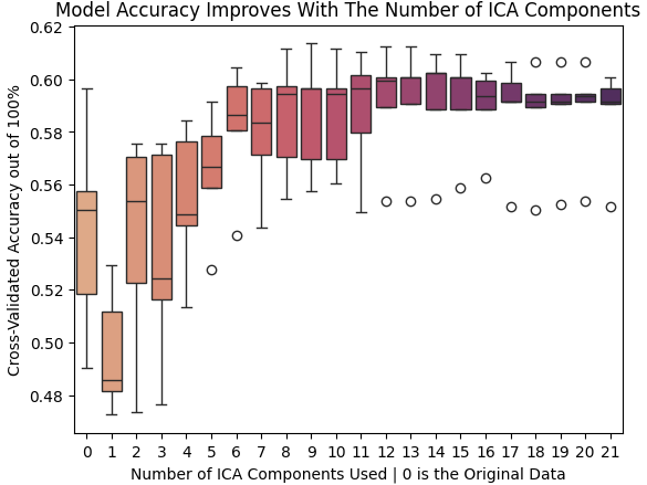
Figure 6: Our performance surpassed the benchmark we established as we increased the number of ICA components to extract from the data.
We will now store the new training manifold created by the ICA algorithm.
ica_transformer = FastICA(n_components=(12))
train_manifold = pd.DataFrame(ica_transformer.fit_transform(train.loc[:,MA]))
The ICA algorithm reduces the size of the correlation matrix. In fact, all pairs of columns produced by the algorithm are uncorrelated. We have plotted the L2 norms of the 2 matrices below. An L2 norm close to 0 informs us that the correlation matrix of the ICA manifold is sparse.
correlation_norms = []

correlation_norms.append(np.linalg.norm(x=train.loc[:,MA].corr(),ord=2))
correlation_norms.append(np.linalg.norm(x=train_manifold.corr(),ord=2))

sns.barplot(correlation_norms)
plt.xticks([0,1],['Original Data','ICA Manifold'])
plt.ylabel('L2 Norm of Correlation Matrix')
plt.xlabel('Input Data')
plt.title('Visualizing the effects of Fast ICA on Data Correlation')
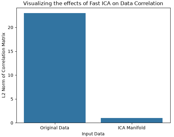
Figure 7: The size of the correlation matrix fell dramatically between the original data and the ICA manifold.
Clustering Our ICA Manifold
Not all the noise in the SMA indicators was filtered out by ICA. We may be curious to understand the distribution of residual noise that leaked into our ICA manifold. It may be possible that there are regions of high and low accuracy in our manifold, or alternatively, noise may be evenly distributed across the ICA manifold. There are many ways to estimate which case is true. One possible way is by using unsupervised clustering algorithms that find high-dimensional groups in our data. These groups are selected to minimize variance within the group and maximize variance across different groups.
from sklearn.cluster import KMeans
We can check for the presence of high-dimensional groups in our ICA manifold that has 12 columns. We instructed the KMeans algorithm to search for 5 groups.
train_manifold.columns = train_manifold.columns.astype(str)
clustering = KMeans(random_state=0,n_clusters=5)
clusters = clustering.fit(train_manifold)
train_manifold['Cluster Labels'] = clusters.labels_
Our interest lies in observing how the model's error rates change across the 5 different groups identified. In future discussions, we may consider how market returns change across the identified clusters. For now, the identification of a group with high accuracy may indicate repeating market conditions under which we excel. The absence of such a group indicates that we may either try using a different clustering algorithm or that our model is stable across the identified market regimes. To get started, we first partitioned our training set into equal halves.
#Partition The Training Set
train_manifold_dev , train_manifold_test =train_manifold.iloc[:train_manifold.shape[0]//2-HORIZON,:] , train_manifold.iloc[train_manifold.shape[0]//2:,:]
Support Vector Machines are well suited for high-dimensional datasets. We will fit the model on the first half of the training set.
model = LSVC()

model.fit(train_manifold_dev,train.loc[0:train_manifold_dev.shape[0]-1,'New Bin Target'])
We then record its errors on the held-out validation half of the training set.
train_manifold_test['Predictions'] = model.predict(train_manifold_test)
train_manifold_test['Predictions'] = np.abs(train_manifold_test['Predictions'] - train.loc[train_manifold_test.shape[0]:,'New Bin Target'])
It appears that the noise was shared almost evenly across all 5 clusters. Only cluster 4 appeared to have a meaningfully low error level. Unfortunately, as we shall see in Figure 9, we notice that the number of observations in cluster 4 was relatively small. Therefore, we cannot exploit this distribution in a material manner.
cluster_noise = []

for i in np.arange(5):
    cluster_noise.append(train_manifold_test.loc[train_manifold_test['Cluster Labels'] == i,'Predictions'].sum() / train_manifold_test.loc[train_manifold_test['Cluster Labels'] == i,'Predictions'].shape[0])

sns.barplot(cluster_noise,palette='flare')
plt.xlabel('KMeans Cluster Labels')
plt.ylabel('Mean Error Levels')
plt.title('Residual Noise In KMean Clusters')
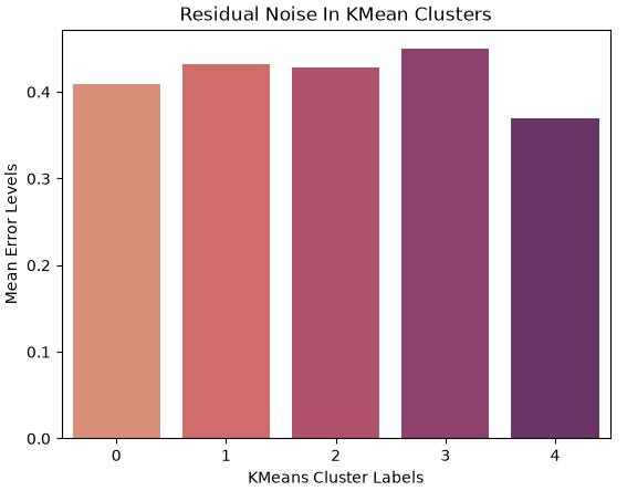
Figure 8: The noise in our ICA manifold was not well separated by unsupervised KMeans clustering.
Cluster 4 has a small population. This makes it unreliable for daily trading needs. If the cluster were more common, we may have been able to exploit the low error rates observed by increasing our trade volume if we forecast that the market will transition to this cluster of good performance. These results could also motivate us to look at other characteristics of the clusters besides model performance. We can consider financial parameters such as the standard deviation of returns, expected return and Sharpe ratio across clusters to gain a different picture.
plt.hist(clusters.labels_)
plt.xlabel('KMeans Cluster Label')
plt.ylabel('Frequency of Observations')
plt.title('Unsupervised Clustering of ICA Components') 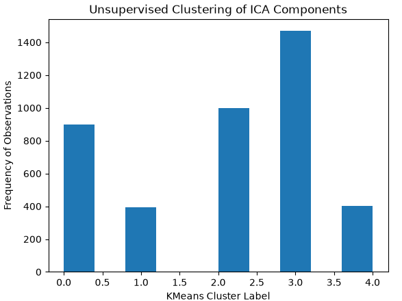
Figure 9: The distribution of our dataset across 5 different KMeans clusters we identified from the ICA manifold.
Parameter Tuning
Now that we have found a good set of inputs for our model, let us now turn our attention to estimating good parameter settings for our model. We will load the RandomizedSearchCV class to help us iterate over different possible parameters. Additionally, we will use the KNeighborsRegressor as our model of choice.
from sklearn.neighbors import KNeighborsRegressor as KNR
from sklearn.model_selection import RandomizedSearchCV
We will initialize the model with a basic shared setting for all instances.
#Initialize the model
#First model learns to encode the data
ica_model = KNR(n_jobs=-1)
Then we define the model settings we wish to iterate over.
#Initialize the parameters to be searched
param_distribution = {
    'n_neighbors':[5,10,15,20,30,50,90,150],
    'weights':['uniform','distance'],
    'algorithm':['auto','ball_tree','kd_tree','brute'],
    'leaf_size':[10,20,30,40,50,60,70,80]
}
Define the randomized search object. There is a tradeoff to be made between the quality of the search and the time taken performing the search. Increasing the number of iterations allowed increases the quality of the search, but this costs more time. The user should feel free to adjust this parameter.
#Initialize the random search object
rscv = RandomizedSearchCV(ica_model,param_distribution,random_state=0,n_iter=90,cv=tscv,n_jobs=-1,scoring='neg_mean_squared_error')
Here are the best settings we found during this search:
#Search
results = rscv.fit(train.loc[:,MA],train_manifold.iloc[:,:12])
results.best_params_
{'weights': 'distance',
'n_neighbors': 150,
'leaf_size': 30,
'algorithm': 'auto'}
We will now fit the model with the best settings we found.
ica_model = KNR(weights='distance',n_neighbors=150,leaf_size=30,algorithm='auto')
ica_model.fit(train.loc[:,MA],train_manifold.iloc[:,:12])
Store the model's predictions. The model we have just trained learned to approximate the ICA manifold from the filtered moving average data. The second model we will build will learn to approximate the change in the indicator from the approximate ICA embeddings.
ica_predictions = pd.DataFrame(ica_model.predict(train.loc[:,MA]))
Let us now create the second model with the same initial settings we used on the prior model.
smoothed_returns_model = KNR(n_jobs=-1) Initialize the randomized search object.
#Initialize the random search object
rscv = RandomizedSearchCV(smoothed_returns_model,param_distribution,random_state=0,n_iter=90,cv=tscv,n_jobs=-1,scoring='neg_mean_squared_error')
Search for the best parameters to predict the target value from approximate ICA components.
#Search
results = rscv.fit(ica_predictions,train.loc[:,'New Target'])
results.best_params_
{'weights': 'uniform',
'n_neighbors': 90,
'leaf_size': 30,
'algorithm': 'ball_tree'}
Fit each model with the best parameters possible.
returns_model = KNR(weights='uniform',n_neighbors=90,leaf_size=30,algorithm='ball_tree',n_jobs=-1)
returns_model.fit(ica_predictions,train.loc[:,'New Target'])
Exporting to ONNX
We are now ready to export our models to ONNX format. ONNX stands for Open Neural Network Exchange; it is an open-source protocol that allows machine learning models to be shared across different programming languages. This allows us to apply our scikit-learn models into our MQL5 applications with ease.
import onnx
from skl2onnx.common.data_types import FloatTensorType
from skl2onnx import convert_sklearn
Next, we will define the input and output shapes of both models we will be exporting.
ica_initial_types = [('float_input',FloatTensorType([1,len(MA)]))]
ica_final_types = [('float_output',FloatTensorType([1,12]))]

returns_initial_types = [('float_input',FloatTensorType([1,12]))]
returns_final_types = [('float_output',FloatTensorType([1,1]))]
Now, we finally save each ONNX model to disk.
onnx_proto = convert_sklearn(ica_model,initial_types=ica_initial_types,final_types=ica_final_types,target_opset=12)
onnx.save(onnx_proto,'EURUSD ICA KNR.onnx')

onnx_proto = convert_sklearn(returns_model,initial_types=returns_initial_types,final_types=returns_final_types,target_opset=12)
onnx.save(onnx_proto,'EURUSD SR KNR.onnx')
Building Our MQL5 Expert Advisor
We will now start building our trading application in MQL5. We will start by importing the trade library to help us manage our position entry.
//+------------------------------------------------------------------+
//|                                                    Filtering.mq5 |
//|                                  Copyright 2026, MetaQuotes Ltd. |
//|                                             https://www.mql5.com |
//+------------------------------------------------------------------+
#property copyright "Copyright 2026, MetaQuotes Ltd."
#property link      "https://www.mql5.com"
#property version   "1.00"

//+------------------------------------------------------------------+
//| Resources                                                        |
//+------------------------------------------------------------------+
#include <Trade\Trade.mqh>
CTrade Trade;
Subsequently, we will load the 2 ONNX models we exported from our Python script.
//+------------------------------------------------------------------+
//| Resources                                                        |
//+------------------------------------------------------------------+
#resource "\\Files\\ICA Filtering\\EURUSD ICA KNR.onnx" as const uchar onnx_ica_proto[];
#resource "\\Files\\ICA Filtering\\EURUSD SR KNR.onnx" as const uchar onnx_returns_proto[];
We will also need a handful of global variables for data that will be shared across many functions in the application.
//+------------------------------------------------------------------+
//| Global variables                                                 |
//+------------------------------------------------------------------+
long        onnx_ica_model,onnx_returns_model;
vectorf     onnx_ica_inputs,onnx_ica_outputs,onnx_return_outputs;
datetime    time_stamp;
int         atr_handler,o_ma_handler,c_ma_handler,h_ma_handler,l_ma_handler;
double      atr[],o_ma[],c_ma[],h_ma[],l_ma[],bid,ask;
Then we will define input variables that our user can adjust to ensure that the application runs with the same settings we used to fetch the market data using our MQL5 script.
//+------------------------------------------------------------------+
//| Input variables                                                 |
//+------------------------------------------------------------------+
input group "Technical Indicators"
input(name="Moving Average Period") int ma_period = 5;
input(name="Moving Average Type") ENUM_MA_METHOD ma_type = MODE_SMA;

input group "Expert Advisor Settings"
input(name="Magic Number") ulong magic_number = 26309;
When our application is set up for the first time, we will set our magic number and load the ONNX models and technical indicators. If something goes wrong when setting either the models or indicators, we will log an error message and fail initialization.
//+------------------------------------------------------------------+
//| Expert initialization function                                   |
//+------------------------------------------------------------------+
int OnInit()
  {
//--- Set the magic number
   Trade.SetExpertMagicNumber(magic_number);

//--- Check if something went wrong
   if(!(LoadOnnxModels()) || !(LoadIndicators()))
     {
      Print("An error occurred during initialization: ",GetLastError());
      return(INIT_FAILED);
     }

//--- Everything was fine
   return(INIT_SUCCEEDED);
  }
If our application is no longer in use, we will call a utility function to clean up the resources we are no longer using. Should an error occur while releasing resources, an error message will be printed to the terminal with the corresponding error code appended.
//+------------------------------------------------------------------+
//| Expert deinitialization function                                 |
//+------------------------------------------------------------------+
void OnDeinit(const int reason)
  {
//--- Free up resources
   if(!ReleaseResources())
     {
      Print("Application failed to shutdown correctly: ",GetLastError());
     }
  }
If new prices are quoted from the broker, we will check for the formation of a new complete daily candle. If a new candle has formed, then we will update our track of time and market prices. In the event of success, we will then proceed to prepare our ONNX model's input data. Assuming that both models' data and forecasts are fetched successfully, then we will look for an entry position that aligns with our model's forecast if we have no open positions.
//+------------------------------------------------------------------+
//| Expert tick function                                             |
//+------------------------------------------------------------------+
void OnTick()
  {
//---
   time_stamp = iTime(Symbol(),PERIOD_D1,1);
   static datetime previous_time_stamp;

   if(previous_time_stamp != time_stamp)
     {
      //--- Update the time stamp
      previous_time_stamp = time_stamp;

      //--- Fetch updated indicator readings
      if(!UpdateMarketData())
        {
         Print("An error occurred while trying to update indicator readings: ",GetLastError());
         return;
        }

      if(!FetchModelData())
        {
         Print("An error occurred while trying to fetch our ONNX model data: ");
         return;
        }

      if(!OnnxRun(onnx_ica_model,ONNX_DATA_TYPE_FLOAT,onnx_ica_inputs,onnx_ica_outputs))
        {
         Print("Failed to approximate ICA embedings: ",GetLastError());
         return;
        }

      else
        {
         if(!OnnxRun(onnx_returns_model,ONNX_DATA_TYPE_FLOAT,onnx_ica_outputs,onnx_return_outputs))
           {

            Print("Failed to forecast market returns: ",GetLastError());
            return;
           }

         else
           {
            SetupPosition();
           }
        }
     }
  }
//+------------------------------------------------------------------+
The following function will allow us to execute our trades if no open trades with our magic number exist.
//+------------------------------------------------------------------+
//| Check if we can enter a position                                 |
//+------------------------------------------------------------------+
void SetupPosition(void)
  {
   if(PositionSelect(Symbol()))
     {
      if(PositionGetInteger(POSITION_MAGIC) != magic_number)
        {
         Print("Attempting to execute trade.");
         EnterTrade();
        }
     }

   else
      if(!PositionSelect(Symbol()))
        {
         Print("Attempting to execute trade.");
         EnterTrade();
        }
  }
Next, we will define the EnterTrade function. This function is responsible for executing trade orders depending on the forecasted, smoothed return that we are anticipating. If the return is expected to be positive, we enter a long position. Otherwise, we enter a short position if the expected return is negative.
//+------------------------------------------------------------------+
//| Execute our trade order                                          |
//+------------------------------------------------------------------+
void EnterTrade(void)
  {
   if(onnx_return_outputs[0] > 0)
     {
      if(!Trade.Buy(0.01,Symbol(),ask,bid-(2*atr[0]),bid+(2*atr[0])))
        {
         Print("Something went wrong while setting up our buy position: ",GetLastError());
         return;
        }
     }

   if(onnx_return_outputs[0] < 0)
     {
      if(!Trade.Sell(0.01,Symbol(),bid,ask+(2*atr[0]),ask-(2*atr[0])))
        {
         Print("Something went wrong while setting up our sell position: ",GetLastError());
         return;
        }
     }
  }
Fetching our model data is straightforward. The float vector is populated with indicator readings and their lags in chronological order, from the previous bar back into the past. This means that the previous bar appears first as the most recent reading, while older bars appear in the last readings. After this is done, we perform a check to ensure that the inputs are valid and not equal to zero.
//+------------------------------------------------------------------+
//| Fetch the input data for our ICA model                           |
//+------------------------------------------------------------------+
bool FetchModelData(void)
  {
//--- Setup model inputs and outputs
//--- ICA Inputs
   onnx_ica_inputs[0] = (float) o_ma[0];
   onnx_ica_inputs[1] = (float) h_ma[0];
   onnx_ica_inputs[2] = (float) l_ma[0];
   onnx_ica_inputs[3] = (float) c_ma[0];
//--- Lag 1
   onnx_ica_inputs[4] = (float) o_ma[1];
   onnx_ica_inputs[5] = (float) h_ma[1];
   onnx_ica_inputs[6] = (float) l_ma[1];
   onnx_ica_inputs[7] = (float) c_ma[1];
//--- Lag 2
   onnx_ica_inputs[8] = (float) o_ma[2];
   onnx_ica_inputs[9] = (float) h_ma[2];
   onnx_ica_inputs[10] = (float) l_ma[2];
   onnx_ica_inputs[11] = (float) c_ma[2];
//--- Lag 3
   onnx_ica_inputs[12] = (float) o_ma[3];
   onnx_ica_inputs[13] = (float) h_ma[3];
   onnx_ica_inputs[14] = (float) l_ma[3];
   onnx_ica_inputs[15] = (float) c_ma[3];
//--- Lag 4
   onnx_ica_inputs[16] = (float) o_ma[4];
   onnx_ica_inputs[17] = (float) h_ma[4];
   onnx_ica_inputs[18] = (float) l_ma[4];
   onnx_ica_inputs[19] = (float) c_ma[4];
//--- Lag 5
   onnx_ica_inputs[20] = (float) o_ma[5];
   onnx_ica_inputs[21] = (float) h_ma[5];
   onnx_ica_inputs[22] = (float) l_ma[5];
   onnx_ica_inputs[23] = (float) c_ma[5];

//--- Validate inputs are not empty
   if(onnx_ica_inputs.Sum() == 0)
     {
      Print("Inputs total equals zero. Something went wrong.");
      return(false);
     }

   return(true);
  }
We will now define the function responsible for updating our technical indicator readings and other market data. The function copies bid and ask prices; on failure, it notifies the user. Otherwise, we move on to copying the technical indicator readings to their respective buffers. Safety checks are performed at every step to ensure that, in the event of failure, trading activities are suspended. The function returns a Boolean flag. It returns false if an error occurs; otherwise, it returns true, indicating that trading can continue.
//+------------------------------------------------------------------+
//| Copy updated market prices                                       |
//+------------------------------------------------------------------+
bool UpdateMarketData(void)
  {
//--- Updated bid and ask prices
   if(!SymbolInfoDouble(Symbol(),SYMBOL_ASK,ask))
     {
      Print("Failed to copy the ask price");
      return(false);
     }

   if(!SymbolInfoDouble(Symbol(),SYMBOL_BID,bid))
     {
      Print("Failed to copy the bid price");
      return(false);
     }
//--- Update technical indicators

//--- High MA

   if(CopyBuffer(h_ma_handler,0,1,6,h_ma) <= 0)
     {
      Print("An error occurred when copying the High moving average buffer: ",GetLastError());
      return(false);
     }
   ArraySetAsSeries(h_ma,true);

//--- Open MA
   if(CopyBuffer(o_ma_handler,0,1,6,o_ma) <= 0)
     {
      Print("An error occurred when copying the Open moving average buffer: ",GetLastError());
      return(false);
     }
   ArraySetAsSeries(o_ma,true);

//--- Low MA
   if(CopyBuffer(l_ma_handler,0,1,6,l_ma) <= 0)
     {
      Print("An error occurred when copying the Low moving average buffer: ",GetLastError());
      return(false);
     }

   ArraySetAsSeries(l_ma,true);

//--- Close MA
   if(CopyBuffer(c_ma_handler,0,1,6,c_ma) <=0)
     {
      Print("An error occurred when copying the Close moving average buffer: ",GetLastError());
      return(false);
     }
   ArraySetAsSeries(c_ma,true);

//--- ATR
   if(CopyBuffer(atr_handler,0,1,6,atr) <=0)
     {
      Print("An error occurred when copying the ATR buffer: ",GetLastError());
      return(false);
     }
   ArraySetAsSeries(atr,true);

   return(true);
  }
Next, we will define the function that loads our technical indicators. This function tests whether all the indicator handles are valid and then returns the appropriate Boolean flag to indicate success or failure. The false flag represents failure. An error message will be given to the user if necessary. The flag returned by the function is used to validate if the application has launched correctly.
//+------------------------------------------------------------------+
//| Setup technical indicators                                       |
//+------------------------------------------------------------------+
bool LoadIndicators(void)
  {
//--- Validate if something went wrong
//--- Technical indicators
   o_ma_handler = iMA(Symbol(),PERIOD_D1,ma_period,0,ma_type,PRICE_OPEN);
   h_ma_handler = iMA(Symbol(),PERIOD_D1,ma_period,0,ma_type,PRICE_HIGH);
   l_ma_handler = iMA(Symbol(),PERIOD_D1,ma_period,0,ma_type,PRICE_LOW);
   c_ma_handler = iMA(Symbol(),PERIOD_D1,ma_period,0,ma_type,PRICE_CLOSE);
   atr_handler  = iATR(Symbol(),PERIOD_D1,14);

   if(atr_handler == INVALID_HANDLE)
     {
      Print("Failed to load the ATR indicator: ",GetLastError());
      return(false);
     }

   if(o_ma_handler == INVALID_HANDLE)
     {
      Print("Failed to load the Open moving average indicator: ",GetLastError());
      return(false);
     }

   if(h_ma_handler == INVALID_HANDLE)
     {
      Print("Failed to load the High moving average indicator: ",GetLastError());
      return(false);
     }

   if(l_ma_handler == INVALID_HANDLE)
     {
      Print("Failed to load the Low moving average indicator: ",GetLastError());
      return(false);
     }

   if(c_ma_handler == INVALID_HANDLE)
     {
      Print("Failed to load the Close moving average indicator: ",GetLastError());
      return(false);
     }

//--- Everything went well
   return(true);
  }
Next, we need a function responsible for setting up our ONNX models. First, this function creates the models from the buffers that we defined in the header and validates that they were created successfully. Once the models have been validated, we attempt to define the input and output shapes for both imported models. Because we use two models, any failure triggers a user-facing error and causes initialization to return false.
//+------------------------------------------------------------------+
//| Prepare our ONNX models for inferencing                          |
//+------------------------------------------------------------------+
bool LoadOnnxModels(void)
  {

//--- ONNX Models
   onnx_ica_model     = OnnxCreateFromBuffer(onnx_ica_proto,ONNX_DATA_TYPE_FLOAT);
   onnx_returns_model = OnnxCreateFromBuffer(onnx_returns_proto,ONNX_DATA_TYPE_FLOAT);

//--- Validate the ONNX model handlers
   if(onnx_returns_model == INVALID_HANDLE)
     {
      return(false);
     }

   if(onnx_ica_model == INVALID_HANDLE)
     {
      return(false);
     }

//--- Validate the ONNX model shapes
   ulong onnx_ica_input_shape[] = {1,24};
   ulong onnx_ica_output_shape[] = {1,12};
   ulong onnx_returns_output_shape[] = {1,1};

   if(!OnnxSetInputShape(onnx_ica_model,0,onnx_ica_input_shape))
     {
      Print("Failed to set the correct ONNX ICA model input shape: ",GetLastError());
      return(false);
     }

   if(!OnnxSetOutputShape(onnx_ica_model,0,onnx_ica_output_shape))
     {
      Print("Failed to set the correct ONNX ICA model output shape: ",GetLastError());
      return(false);
     }

   if(!OnnxSetInputShape(onnx_returns_model,0,onnx_ica_output_shape))
     {
      Print("Failed to set the correct ONNX smoothed returns model input shape: ",GetLastError());
      return(false);
     }

   if(!OnnxSetOutputShape(onnx_returns_model,0,onnx_returns_output_shape))
     {
      Print("Failed to set the correct ONNX smoothed returns model output shape: ",GetLastError());
      return(false);
     }

//--- Prepare ONNX model I/O
   onnx_ica_inputs = vectorf::Zeros(24);
   onnx_ica_outputs = vectorf::Zeros(12);
   onnx_return_outputs = vectorf::Zeros(1);

//--- Everything went well
   return(true);
  }
Lastly, we define a function responsible for releasing all the resources dedicated to the indicators and ONNX models that our trading strategy relies on. This function is called when the application is no longer being used by the deinitialization event handler, ensuring that all allocated resources are properly released.
//+------------------------------------------------------------------+
//| Free up all resources we are no longer using                     |
//+------------------------------------------------------------------+
bool ReleaseResources(void)
  {
   if(!OnnxRelease(onnx_ica_model))
     {
      Print("An error occurred when releasing the ONNX ICA model: ",GetLastError());
      return(false);
     }

   if(!OnnxRelease(onnx_returns_model))
     {
      Print("An error occurred when releasing the ONNX Smoothed Returns model: ",GetLastError());
      return(false);
     }

   if(!IndicatorRelease(atr_handler))
     {
      Print("An error occurred while trying to release the ATR Indicator: ",GetLastError());
      return(false);
     }

   if(!IndicatorRelease(o_ma_handler))
     {
      Print("An error occurred while releasing the Open Moving Average Indicator");
      return(false);
     }

   if(!IndicatorRelease(l_ma_handler))
     {
      Print("An error occurred while releasing the Low Moving Average Indicator");
      return(false);
     }

   if(!IndicatorRelease(h_ma_handler))
     {
      Print("An error occurred while releasing the High Moving Average Indicator");
      return(false);
     }

   if(!IndicatorRelease(c_ma_handler))
     {
      Print("An error occurred while releasing the Close Moving Average Indicator");
      return(false);
     }
   return(true);
  }
//+------------------------------------------------------------------+
Testing Our Trading Strategy
Our strategy will be tested over an out-of-sample window that our ONNX model did not train over during its construction. The test will run 3 years, spanning from 2023 until 2026. Due to the limited dataset available from our broker, the test sample size was constrained. The reader is advised to use more data if they can access it from their broker over the network.
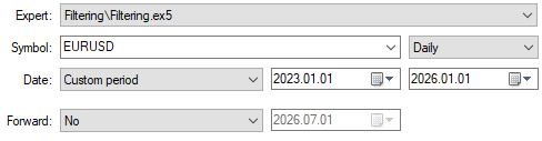
Figure 10: The out-of-sample backtest window we will use to evaluate our trading strategy.
Let us test our application under realistic conditions. We will do this by modeling our ticks based on real ticks and preferring random delay settings. These settings mimic live trading conditions that can be noisy.
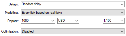
Figure 11: The backtest will be performed under realistic settings to emulate real trading scenarios.
The trading strategy had an accuracy of 56% on the out-of-sample period. This is reasonably aligned with the accuracy of 59% that we obtained when we cross-validated the model in Python over the training period. We produced a Sharpe Ratio of 0.62, which demonstrates that the application may warrant further development.
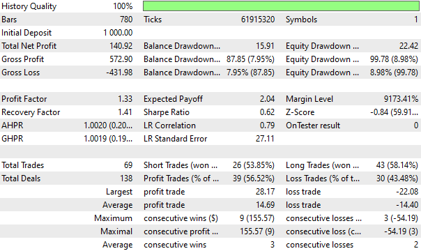
Figure 12: The detailed statistical results produced by our trading strategy.
The equity curve produced by the trading strategy is captured in Figure 12 below. The strategy appears to have a positive trend in the account balance over time. If these results can be validated over longer horizons in our next discussion, then we may have the foundation of a good strategy.
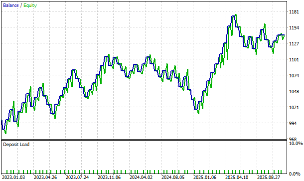
Figure 13: The performance of our trading strategy plotted against time.
Conclusion
After reading this article, the reader walks away with an ensemble strategy for handling market noise. Although we have discussed the potential benefits of the proposed solution throughout the article, we must also review some of its possible weaknesses. The first limitation of our strategy is that the test was limited to a small out-of-sample period. This means that our results could vary if we repeat the test over more data.
Moreover, ICA is a linear source separation technique. This means it makes rigid assumptions about the process generating the independent sources. These assumptions could be violated during real market conditions; if this is the case, the performance of the strategy deteriorates, and no warnings are given. Additionally, this strategy contains many tunable parameters, yet we tuned only a few of the available options. For example, the source separation technique itself is a tunable parameter. Besides ICA, there are other source separation and clustering algorithms that we did not consider besides ICA and KMeans.
Lastly, relying on two models to forecast our target introduces a compounding effect. Errors from the first model (ICA embedding approximation) can propagate to the second model and compound the overall error. As a result, a feedback system of noise may be inadvertently created, and our current solution does not account for or correct this behavior. This is the trade-off we accept to avoid the meticulous and demanding task of implementing the ICA algorithm from scratch in native MQL5, although this is certainly a worthwhile task for future work.
All in all, the article aims to present a balanced perspective on how we can explore problems as difficult to understand as market noise from a statistical perspective.
| File name | File description |
|---|---|
| Filtering.mq5 | The trading application we built in this discussion. It is located inside the Experts subfolder in the attached file. |
| EURUSD_ICA_KNR.onnx | This is the ONNX model responsible for approximating the corresponding ICA embeddings from filtered SMA data. |
| EURUSD_SR_KNR.onnx | Our ONNX model that forecasted smoothed returns from the output of the first model. Both models are housed in the Files subfolder. |
| Noise_Filter.mq5 | The MQL5 script we built to fetch the market data we needed. The script is found in the Scripts subfolder. |
| eurusd-statistical-noise-filter.ipynb | The Jupyter Notebook we built to analyze the market data we fetched from the MetaTrader 5 Terminal. The notebook is contained inside the Files subfolder. It sits in the same folder as the ONNX files, but in its own Notebook folder. |
Warning: All rights to these materials are reserved by MetaQuotes Ltd. Copying or reprinting of these materials in whole or in part is prohibited.
This article was written by a user of the site and reflects their personal views. MetaQuotes Ltd is not responsible for the accuracy of the information presented, nor for any consequences resulting from the use of the solutions, strategies or recommendations described.

 MQL5 Bootstrap (III): Simplified Functions for Working with News
 Differential Search Algorithm (DSA)
 Fast Integration of a Large Language Model with MetaTrader 5 (Part II): Fine-Tuning on Real Data, Backtesting, and Live Trading by the Model
 Neural Networks in Trading: Probabilistic Time Series Forecasting (K2VAE)

- Free trading apps
- Over 8,000 signals for copying
- Economic news for exploring financial markets
You agree to website policy and terms of use