Functions for activating neurons during training: The key to fast convergence?

Introduction

In the previous article we examined the properties of a simple MLP neural network as an approximator (reinforcement learning) in trading. In this case, no special attention was paid to the properties of the activation functions, but the popular hyperbolic tangent sigmoid was used. Also in one of the articles we discussed the capabilities of the well-known and widely used ADAM algorithm. I modified it into an independent population method of the ADAMm global optimization .

In this article, we will delve into the capabilities of a neural network as a data interpolator (supervised learning), focusing on the properties of neuron activation functions. We will use the ADAM optimization algorithm built into the neural network (as is usually done in the application of neural networks) and conduct research on the influence of the activation function and its derivative on the convergence rate of the optimization algorithm.

Imagine a river with many tributaries. In its normal state, water flows freely, creating a complex pattern of currents and whirlpools. But what happens if we start building a system of locks and dams? We will be able to control the flow of water, direct it in the right direction and regulate the strength of the current. The activation function in neural networks plays a similar role: it decides which signals to pass through and which to delay or attenuate. Without it, a neural network would be just a set of linear transformations.

The activation function adds dynamics to the neural network operation, allowing it to capture subtle nuances in the data. For example, in a face recognition task, an activation function helps the network notice tiny details, such as the arch of an eyebrow or the shape of a chin. The correct choice of activation function affects how a neural network performs on various tasks. Some features are better suited for the early stages of training, providing clear and understandable signals. Other features allow the network to pick up more subtle patterns at advanced stages, while others sort out the unnecessary ones, leaving only the most important.

If we do not know the properties of activation functions, we may run into problems. A neural network may begin to "stumble" on simple tasks or "overlook" important details. The main purpose of activation functions is to introduce nonlinearity into the neural network and normalize the output values.

The aim of this article is to identify the issues associated with the use of different activation functions and their impact on the accuracy of a neural network in traversing example points (interpolation) while minimizing error. We will also find out whether activation functions actually affect the convergence rate, or whether this is a property of the optimization algorithm used. As a reference algorithm, we will use a modified population ADAMm that uses elements of stochasticity, and conduct tests with the ADAM built into MLP (classical usage). The latter should intuitively have an advantage, since it has direct access to the gradient of the fitness function surface thanks to the derivative of the activation function. At the same time, the population stochastic ADAMm has no access to the derivative and has no idea at all about the optimization problem surface. Let's see what comes out of this and draw some conclusions.

The article is of an exploratory nature and the narrative proceeds in the order of an experiment.

Implementation of MLP neural network with embedded ADAM

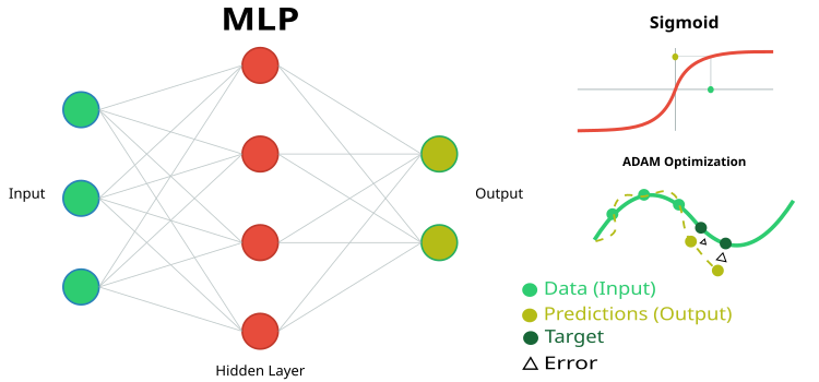
Figure 1. Schematic representation of the MLP neural network and its training

To conduct the current study, we will need a simple and transparent MLP neural network code, without using specialized matrix calculations built into the MQL5 language. This will allow us to clearly understand what exactly is happening in the logic of the neural network, as well as to understand what certain results depend on.

We will implement a multilayer perceptron (MLP) with a built-in ADAM (Adaptive Moment Estimation) optimization algorithm. A class and structure represent a part of a neural network implementation, in which the main components are defined: neurons, neuron layers, and weights.

1. The C_Neuro class represents a neuron, which is the basic unit in a neural network.

• C_Neuron() is a constructor that initializes the values of the "m" and "v" properties to zero. These values are used for the optimization algorithm.
• out — the output value of the neuron after applying the activation function.
• delta — the error delta used to calculate the gradient during training.
• bias — a bias value added to the neuron inputs.
• m and v are used to store the first and second moments for the bias, used by the ADAM optimization method.

2. The S_NeuronLayer structure represents a layer of neurons. C_Neuron n [] is an array of neurons in a neural network layer.

To store weights between neurons, we use an object-oriented approach instead of simple two-dimensional arrays. It is based on the C_Weight class, which stores not only the connection weight itself, but also the optimization parameters - the first and second moments used in the ADAM algorithm. The data structure is arranged hierarchically: S_WeightsLayer contains an array of S_WeightsLayerR structures, which in turn contain arrays of C_Weight objects. This makes it easy to address any weight in the network through a clear index chain.

For example, to refer to the weight of the connection between the first neuron of layer 0 and the second neuron of the next layer, we use the notation: wL [0].nOnL [1].nOnR [2].w. Here the first index indicates a pair of adjacent layers, the second indicates a neuron in the left layer, and the third indicates a neuron in the right layer.

//——————————————————————————————————————————————————————————————————————————————
// Neuron class
class C_Neuron
{
  public:
  C_Neuron ()
  {
    m = 0.0;
    v = 0.0;
  }
  double out;   // Neuron output after the activation function
  double delta; // Error delta
  double bias;  // Bias
  double m;     // First moment of displacement
  double v;     // Second moment of displacement
};
//——————————————————————————————————————————————————————————————————————————————

//——————————————————————————————————————————————————————————————————————————————
// Structure of the neuron layer
struct S_NeuronLayer
{
    C_Neuron n []; // neurons in the layer
};
//——————————————————————————————————————————————————————————————————————————————

//——————————————————————————————————————————————————————————————————————————————
// Weight class
class C_Weight
{
  public:
  C_Weight ()
  {
    w = 0.0;
    m = 0.0;
    v = 0.0;
  }

  double w; // Weight
  double m; // First moment
  double v; // Second moment
};
//——————————————————————————————————————————————————————————————————————————————

//——————————————————————————————————————————————————————————————————————————————
//Weight structure for neurons on the right
struct S_WeightsLayerR
{
    C_Weight nOnR [];
};
//——————————————————————————————————————————————————————————————————————————————

//——————————————————————————————————————————————————————————————————————————————
//Weight structure for neurons on the left
struct S_WeightsLayer
{
    S_WeightsLayerR nOnL [];
};
//——————————————————————————————————————————————————————————————————————————————

The C_MLPa multilayer perceptron (MLP) class implements the basic functions of a neural network, including forward pass and backpropagation learning using the ADAM optimization algorithm. Let's take a look at what it can do:

Network structure:

• The network consists of successive layers: input -> hidden layers -> output layer.
• Each neuron in a layer is connected to all neurons in the next layer (fully connected network).

Key features:

• Init is a method for creating a network with a given configuration.
• ImportWeights and ExportWeights — loading and saving network weights.
• ForwProp - forward pass: obtaining the network response to the input data.
• BackProp - network training method based on backpropagation of errors.

Training parameters (ADAM algorithm):

• alpha (0.001) — how fast the network learns.
• beta1 (0.9) and beta2 (0.999) — parameters that help the network learn consistently.
• epsilon (1e-8) — a small number to protect against division by zero.

Internal components:

• BackProp stores information about the size of each layer (layersSize).
• It contains all neurons (nL) and weights between them (wL),
• as well as keeps track of the number of weights (wC) and layers (nLC).
• actFunc uses the selected activation function.
  

Essentially, this class is the "brain" of a neural network, which can accept input data, process it through a system of neurons and weights, produce a result, and learn from its mistakes, gradually improving the accuracy of its predictions.

//+-----------------------------------------------------------------------------------------+
//| Multilayer Perceptron (MLP) class                                                       |
//| Implements forward pass through a fully connected neural network and training using the |
//| backpropagation of error by ADAM optimization algorithm                                 |
//| Architecture: Lin -> L1 -> L2 -> ... Ln -> Lout                                         |
//+-----------------------------------------------------------------------------------------+
class C_MLPa
{
  public: //--------------------------------------------------------------------
  ~C_MLPa ()
  {
    delete actFunc;
  }
  C_MLPa ()
  {
    alpha   = 0.001;   // Training speed
    beta1   = 0.9;     // Decay ratio for the first moment
    beta2   = 0.999;   // Decay ratio for the second moment
    epsilon = 1e-8;    // Small constant for numerical stability
  }

  // Network initialization with the given configuration, Returns the total number of weights in the network, or 0 in case of an error
  int    Init          (int &layerConfig [], int actFuncType, int seed);
  bool   ImportWeights (double &weights []);  // Import weights
  bool   ExportWeights (double &weights []);  // Export weights

  // Forward pass through the network
  void   ForwProp (double &inLayer  [],  // input values
                   double &outLayer []); // output layer values

  // Error backpropagation with ADAM optimization algorithm
  void   BackProp (double &errors []);

  // Get the total number of weights in the network
  int    GetWcount () { return wC; }

  // ADAM optimization parameters 
  double alpha;          // Training speed
  double beta1;          // Decay ratio for the first moment
  double beta2;          // Decay ratio for the second moment
  double epsilon;        // Small constant for numerical stability

  int layersSize    [];  // Size of each layer (number of neurons)
  S_NeuronLayer  nL [];  // Layers of neurons, example of access: nLayers [].n [].a
  S_WeightsLayer wL [];  // Layers of weights between layers of neurons, example of access: wLayers [].nOnLeft [].nOnRight [].w

  private: //-------------------------------------------------------------------
  int            wC;       // Total number of weights in the network (including biases)
  int            nLC;      // Total number of neuron layers (including input and output ones)
  int            wLC;      // Total number of weight layers (between neuron layers)
  int            t;        // Iteration counter
  C_Base_ActFunc *actFunc; // Activation functions and their derivatives
};
//——————————————————————————————————————————————————————————————————————————————

The Init method initializes the multilayer perceptron structure by setting the number of neurons in each layer, choosing the activation function, and generating initial weights for the neurons. It checks the validity of the network configuration and returns the total number of required weights or 0 in case of an error.

Parameters:

• layerConfig [] — array containing the number of neurons in each network layer.
• actFuncType — type of activation function to be used in the neural network (e.g. sigmoid, etc.).
• seed — a seed that initializes a number for the random number generator, which allows for reproducible results when initializing weights.

Operation Logic:

1. The method determines the number of layers based on the passed layerConfig array.
2. It ensure that the number of layers is at least 2, and that each layer contains a positive number of neurons. If an error occurs, it displays a message and terminates execution.
3. The method copies the layer sizes to the layersSize array and initializes the arrays for storing neurons and weights.
4. It calculates the total number of weights required to connect neurons between layers.
5. Besides, it initializes weights using the Xavier method, which theoretically helps avoid problems with gradient decaying or exploding.
6. Depending on the passed activation function type, the method creates a corresponding activation function object.
7. It initializes the iteration counter to zero, used in the ADAM algorithm.
   

//+----------------------------------------------------------------------------+
//| Initialize the network                                                     |
//| layerConfig - array with the number of neurons in each layer               |
//| Returns the total number of weights needed, or 0 in case of an error       |
//+----------------------------------------------------------------------------+
int C_MLPa::Init (int &layerConfig [], int actFuncType, int seed)
{
  nLC = ArraySize (layerConfig);

  if (nLC < 2)
  {
    Print ("Network configuration error! Less than 2 layers!");
    return 0;
  }

  // Check configuration
  for (int i = 0; i < nLC; i++)
  {
    if (layerConfig [i] <= 0)
    {
      Print ("Network configuration error! Layer #" + string (i + 1) + " contains 0 neurons!");
      return 0;
    }
  }

  wLC = nLC - 1;
  ArrayCopy (layersSize, layerConfig, 0, 0, WHOLE_ARRAY);

  // Initialize neuron layers
  ArrayResize (nL, nLC);
  for (int i = 0; i < nLC; i++)
  {
    ArrayResize (nL [i].n, layersSize [i]);
  }

  // Initialize weight layers
  ArrayResize (wL, wLC);
  for (int w = 0; w < wLC; w++)
  {
    ArrayResize (wL [w].nOnL, layersSize [w]);
    for (int n = 0; n < layersSize [w]; n++)
    {
      ArrayResize (wL [w].nOnL [n].nOnR, layersSize [w + 1]);
    }
  }

  // Calculate the total number of weights
  wC = 0;
  for (int i = 0; i < nLC - 1; i++) wC += layersSize [i] * layersSize [i + 1] + layersSize [i + 1];

  // Initialize weights
  double weights [];  ArrayResize (weights, wC);

  srand (seed);
  
  //Xavier: U(-√(6/(n₁+n₂)), √(6/(n₁+n₂)))
  double n = sqrt (6.0 / (layersSize [0] + layersSize [nLC - 1]));
  for (int i = 0; i < wC; i++)
  {
    weights [i] = (2.0 * n) * (rand () / 32767.0) - n;
  }

  ImportWeights (weights);

  switch (actFuncType)
  {
    case eActACON:      actFunc = new C_ActACON      (); break;
    case eActAlgSigm:   actFunc = new C_ActAlgSigm   (); break;
    case eActBentIdent: actFunc = new C_ActBentIdent (); break;
    case eActRatSigm:   actFunc = new C_ActRatSigm   (); break;
    case eActSiLU:      actFunc = new C_ActSiLU      (); break;
    case eActSoftPlus:  actFunc = new C_ActSoftPlus  (); break;
    default:            actFunc = new C_ActTanh      (); break;
  }

  t = 0;
  return wC;
}
//——————————————————————————————————————————————————————————————————————————————

Let's look further at two methods - ImportWeights and ExportWeights. These methods are designed to import and export weights and biases of a multilayer perceptron. ImportWeights is responsible for importing weights and biases from the "weights" array into the neural network structure.

First, the method checks whether the size of the passed "weights" array matches the number of weights stored in the wC variable. If the sizes do not match, the method returns 'false' indicating an error.

The wCNT variable is used to track the current index in the "weights" array.
Loops through layers and neurons:

• The outer loop iterates through each layer, starting with the second one (index 1), since the first layer is the input layer and has no weights or biases.
• The inner loop iterates over each neuron in the current layer.
• For each neuron, the "bias" value is set from the "weights" array, and the wCNT counter is incremented.
• A nested loop iterates through all the neurons in the previous layer, setting the weights that connect the neurons in the current layer to the neurons in the previous layer.

ExportWeights — the method is responsible for exporting weights and biases from the neural network structure to the "weights" array. The method logic is similar to that of the ImportWeights method. Both of these methods allow saving weights and biases in an external program in relation to the network class, use the trained network in the future, and also allow the use of external optimization algorithms, such as population ones.

//+----------------------------------------------------------------------------+
//| Import network weights and biases                                          |
//+----------------------------------------------------------------------------+
bool C_MLPa::ImportWeights (double &weights [])
{
  if (ArraySize (weights) != wC) return false;

  int wCNT = 0;

  for (int ln = 1; ln < nLC; ln++)
  {
    for (int n = 0; n < layersSize [ln]; n++)
    {
      nL [ln].n [n].bias = weights [wCNT++];

      for (int w = 0; w < layersSize [ln - 1]; w++)
      {
        wL [ln - 1].nOnL [w].nOnR [n].w = weights [wCNT++];
      }
    }
  }

  return true;
}
//——————————————————————————————————————————————————————————————————————————————

//+----------------------------------------------------------------------------+
//| Export network weights and biases                                          |
//+----------------------------------------------------------------------------+
bool C_MLPa::ExportWeights (double &weights [])
{
  ArrayResize (weights, wC);

  int wCNT = 0;

  for (int ln = 1; ln < nLC; ln++)
  {
    for (int n = 0; n < layersSize [ln]; n++)
    {
      weights [wCNT++] = nL [ln].n [n].bias;

      for (int w = 0; w < layersSize [ln - 1]; w++)
      {
        weights [wCNT++] = wL [ln - 1].nOnL [w].nOnR [n].w;
      }
    }
  }

  return true;
}
//——————————————————————————————————————————————————————————————————————————————

The ForwProp method (forward pass) sequentially calculates the values of all layers of a multilayer perceptron from the input layer to the output one. It takes input values, handles them through hidden layers and generates output values. Parameters:

• inLayer [] - array of input values for the neural network (in green in Figure 1).
• outLayer [] - array the values of the output layer will be set into after handling (in yellow in Figure 1).
  

The method initializes activation values for the input layer neurons by copying the input values from the inLayer array to the corresponding neurons.

Handling hidden and output layers:

• The outer loop iterates through all layers, starting from the second one (index 1), since the first layer is the input one.
• The inner loop goes through each neuron of the current layer.
• For each neuron, the sum of the weighted inputs is calculated:
• It starts by adding a bias to the neuron.
• The nested loop iterates through all neurons of the previous layer, adding to "val" the product of the output value of the neuron of the previous layer and the corresponding weight.
• After calculating the sum, the activation function is applied to "val", and the result is stored in the output value of the current layer neuron.

After handling all layers, the method copies the output values from the last layer (the output layer) into the outLayer array.

//+----------------------------------------------------------------------------+
//| Direct network pass                                                        |
//| Calculate the values of all layers sequentially from input to output       |
//+----------------------------------------------------------------------------+
void C_MLPa::ForwProp (double &inLayer  [],  // input values
                       double &outLayer [])  // output layer values
{
  double val;

  // Set the input layer activation values
  for (int n = 0; n < layersSize [0]; n++)
  {
    nL [0].n [n].out = inLayer [n];
  }

  // Handle hidden and output layers
  for (int ln = 1; ln < nLC; ln++)
  {
    for (int n = 0; n < layersSize [ln]; n++)
    {
      val = nL [ln].n [n].bias;

      for (int w = 0; w < layersSize [ln - 1]; w++)
      {
        val += nL [ln - 1].n [w].out * wL [ln - 1].nOnL [w].nOnR [n].w;
      }

      nL [ln].n [n].out = actFunc.Activ (val); // Apply activation function
    }
  }

  // Set the output layer values
  for (int n = 0; n < layersSize [nLC - 1]; n++) outLayer [n] = nL [nLC - 1].n [n].out;
}
//——————————————————————————————————————————————————————————————————————————————

The BackProp method implements backpropagation of errors in a multilayer perceptron. It updates the weights and biases of all layers from output to input using the ADAM optimization algorithm. Operation Logic:

The "t" variable is incremented to keep track of the number of iterations and is used in the ADAM logic equation.

Calculating deltas for all layers:

• The outer loop iterates through the layers in reverse order, starting with the output layer and ending with the input one.
• The inner loop goes through the neurons of the current layer.
• If the current layer is the output one, the delta is calculated as the product of the error (errors[nCurr]) and the derivative of the activation function for the output neuron.
• For hidden layers, the delta is calculated as the sum of the products of the deltas of the next layer and the corresponding weights.
• The delta is then adjusted by the derivative of the activation function, and the result is stored in nL [ln].n [nCurr].delta.

Updating biases using ADAM:

• The outer loop goes through all layers, starting from the second one.
• For each neuron of the current layer, the bias moments "m" and "v" are updated using the beta1 and beta2 parameters.
• Then the m_hat and v_hat displacement moments are adjusted.
• Finally, the bias is updated using the adjusted moments.

Updating weights using ADAM:

• The outer loop goes through all weight layers.
• Inner loops go through the neurons of the current layer and the next layer.
• For each weight, a gradient is calculated, which is then used to update the "m" and "v" moments.
• After adjusting the m_hat and v_hat weight moments, the weights are updated using the adjusted moments.

//+----------------------------------------------------------------------------+
//| Backward network pass                                                      |
//| Update the weights and biases of all layers from output to input           |
//+----------------------------------------------------------------------------+
void C_MLPa::BackProp (double &errors [])
{
  t++;  // Increase the iteration counter

  double delta;     // current neuron delta
  double deltaNext; // delta of the neuron in the next layer connected to the current neuron
  double out;       // neuron value after applying the activation function
  double deriv;     // derivative
  double w;         // weight for connecting the current neuron to the neuron of the next layer

  // 1. Calculating deltas for all layers ----------------------------------------
  for (int ln = nLC - 1; ln > 0; ln--)                  // walk through layers in reverse order from output to input
  {
    for (int nCurr = 0; nCurr < layersSize [ln]; nCurr++)        // iterate through the neurons of the current layer
    {
      if (ln == nLC - 1)
      {
        delta = errors [nCurr] * actFunc.Deriv (nL [ln].n [nCurr].out);
      }
      else
      {
        delta = 0.0;

        // Sum the products of the deltas of the next layer by the corresponding weights
        for (int nNext = 0; nNext < layersSize [ln + 1]; nNext++) // pass the neurons of the next layer in the usual order
        {
          deltaNext = nL [ln + 1].n [nNext].delta;
          w         = wL [ln].nOnL [nCurr].nOnR [nNext].w;
          delta    += deltaNext * w;
        }
      }

      // Delta considering the derivative of the sigmoid
      out   = nL [ln].n [nCurr].out;
      deriv = actFunc.Deriv (out);
      nL [ln].n [nCurr].delta = delta * deriv;
    }
  }

  // 2. Update biases using ADAM ------------------------------
  for (int ln = 1; ln < nLC; ln++)
  {
    for (int nCurr = 0; nCurr < layersSize [ln]; nCurr++)
    {
      delta = nL [ln].n [nCurr].delta;

      // Update displacement moments
      nL [ln].n [nCurr].m = beta1 * nL [ln].n [nCurr].m + (1.0 - beta1) * delta;
      nL [ln].n [nCurr].v = beta2 * nL [ln].n [nCurr].v + (1.0 - beta2) * delta * delta;

      // Adjust displacement moments
      double m_hat = nL [ln].n [nCurr].m / (1.0 - pow (beta1, t));
      double v_hat = nL [ln].n [nCurr].v / (1.0 - pow (beta2, t));

      // Update bias
      nL [ln].n [nCurr].bias += alpha * m_hat / (sqrt (v_hat) + epsilon);
    }
  }

  // 3. Update weights using ADAM ---------------------------------
  for (int lw = 0; lw < wLC; lw++)
  {
    for (int nCurr = 0; nCurr < layersSize [lw]; nCurr++)
    {
      for (int nNext = 0; nNext < layersSize [lw + 1]; nNext++)
      {
        deltaNext = nL [lw + 1].n [nNext].delta;
        out       = nL [lw].n [nCurr].out;
        double gradient = deltaNext * out;

        // Update moments for weights
        wL [lw].nOnL [nCurr].nOnR [nNext].m = beta1 * wL [lw].nOnL [nCurr].nOnR [nNext].m + (1.0 - beta1) * gradient;
        wL [lw].nOnL [nCurr].nOnR [nNext].v = beta2 * wL [lw].nOnL [nCurr].nOnR [nNext].v + (1.0 - beta2) * gradient * gradient;

        // Adjust weight moments
        double m_hat = wL [lw].nOnL [nCurr].nOnR [nNext].m / (1.0 - pow (beta1, t));
        double v_hat = wL [lw].nOnL [nCurr].nOnR [nNext].v / (1.0 - pow (beta2, t));

        // Update weight
        wL [lw].nOnL [nCurr].nOnR [nNext].w += alpha * m_hat / (sqrt (v_hat) + epsilon);
      }
    }
  }
}
//——————————————————————————————————————————————————————————————————————————————

Code for the stand for rendering activation functions

The stand is designed for testing the correct operation of various activation functions used in neural networks, as well as for displaying them in the form of a graph. The resulting images are used later in the article to visually assess their appearance. The code is quite simple and there is no particular point in describing it.

#include <Graphics\Graphic.mqh>
#include <Math\AOs\NeuroNets\MLPa.mqh>

#define SIZE_X 750
#define SIZE_Y 200

//--- input parameters
input E_Act ACT = eActTanh;
input int   CNT = 10000;

//——————————————————————————————————————————————————————————————————————————————
void OnStart ()
{
  ObjectDelete (ChartID (), "Test");
  double activ [];
  double deriv [];

  //----------------------------------------------------------------------------
  C_Base_ActFunc *act;
  switch (ACT)
  {
    default:            act = new C_ActTanh      (); break;
    case eActAlgSigm:   act = new C_ActAlgSigm   (); break;
    case eActRatSigm:   act = new C_ActRatSigm   (); break;
    
    case eActSoftPlus:  act = new C_ActSoftPlus  (); break;
    case eActBentIdent: act = new C_ActBentIdent (); break;
    case eActSiLU:      act = new C_ActSiLU      (); break;
    
    case eActACON:      act = new C_ActACON      (); break;
    case eActSnake:     act = new C_ActSnake     (); break;
    case eActSERF:      act = new C_ActSERF      (); break;
  }
  
  //----------------------------------------------------------------------------
  ActFuncTest (act, activ, deriv, CNT, -10, 10);
  
  //----------------------------------------------------------------------------
  CGraphic gr_test;
  gr_test.Create (0, "Test", 0, 0, 20, SIZE_X, SIZE_Y + 20);
  gr_test.YAxis ().Name (act.GetFuncName () + ": Value");
  gr_test.YAxis ().NameSize (13);
  gr_test.HistorySymbolSize (10);
  gr_test.CurveAdd (activ, ColorToARGB (clrRed,  255), CURVE_LINES, "activ");
  gr_test.CurveAdd (deriv, ColorToARGB (clrBlue, 255), CURVE_LINES, "deriv");
  gr_test.CurvePlotAll ();
  gr_test.Redraw (true);
  gr_test.Update ();
  
  //----------------------------------------------------------------------------
  delete act;
}
//——————————————————————————————————————————————————————————————————————————————

//——————————————————————————————————————————————————————————————————————————————
void ActFuncTest (C_Base_ActFunc &act, double &arrayAct [], double &arrayDer [], int testCount, double min, double max)
{
  Print (act.GetFuncName (), " [", min, "; ", max, "]");
  Print (act.Activ (min), " ", act.Activ (0), " ", act.Activ (max));
  Print (act.Deriv (min), " ", act.Deriv (0), " ", act.Deriv (max));

  ArrayResize (arrayAct, testCount);
  ArrayResize (arrayDer, testCount);
  double x    = 0.0;
  double step = (max - min) / testCount;
  
  for (int i = 0; i < testCount; i++)
  {
    x = min + step * i;

    arrayAct [i] = act.Activ (x);
    arrayDer [i] = act.Deriv (x);
  }
}
//——————————————————————————————————————————————————————————————————————————————

Code of activation function classes

There are many different neuron activation functions used in a variety of neural network problems. I tried to select functions that include both the well-known hyperbolic tangent and lesser-known ones, such as the Snake activation function, while excluding functions that are very similar in appearance and properties. They can be conditionally divided into three groups:

1. Sigmoid functions,
2. Nonlinear switches,
3. Periodic functions.

Implement the C_Base_ActFunc base class for neuron activation functions. It contains two virtual functions: Activ to calculate the activation and Deriv to calculate the derivative. The GetFuncName() method returns the name of the activation function stored in the funcName protected cell. The class is intended to be inherited to create concrete implementations of activation functions. By creating the activation function object, we can speed up calculations by eliminating the need for multiple uses of "if" and "switch".

//——————————————————————————————————————————————————————————————————————————————
// Base class of the neuron activation function
class C_Base_ActFunc
{
  public:
  virtual double Activ (double inp) = 0; // Virtual activation function
  virtual double Deriv (double inp) = 0; // Virtual derivative function
  string         GetFuncName () {return funcName;}
  protected:
  string funcName;
};
//——————————————————————————————————————————————————————————————————————————————

The C_ActTanh class implements the hyperbolic tangent activation function and its derivative and inherits from the C_Base_ActFunc base class. In the class constructor, the activation function name is set to ActTanh in the funcName variable. Activation method:

• Activ (double x) calculates the value of the hyperbolic tangent activation function using the equation: f(x) = 2 / (1 + exp ( − 2  ⋅  (x)) − 1. This equation converts the "x" input to the range from -1 to 1.

Derivative method:

• Deriv(double x) computes the derivative of the activation function. The derivative of the hyperbolic tangent is expressed as: f′(x) = 1 − (f (x)) ^ 2, where f(x) is the value of the activation function computed for the current "x". The derivative shows how quickly a function changes with respect to the input value.

//——————————————————————————————————————————————————————————————————————————————
// Hyperbolic tangent
class C_ActTanh : public C_Base_ActFunc
{
  public:
  C_ActTanh () {funcName = "ActTanh";}

  double Activ (double x)
  {
    return 2.0 / (1.0 + exp (-2 * (x))) - 1.0;
  }

  double Deriv (double x)
  {
    //1 - (f(x))^2
    double fx = Activ (x);
    return 1.0 - fx * fx;
  }
};
//——————————————————————————————————————————————————————————————————————————————

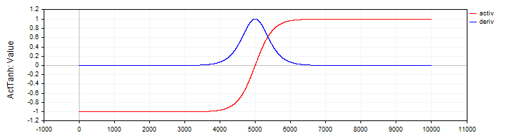
Figure 2. Hyperbolic tangent and its derivative

The C_ActAlgSigm class, similar to the C_ActTanh class, implements the algebraic sigmoid as an activation function with methods for calculating the activation and its derivative.

//——————————————————————————————————————————————————————————————————————————————
// Algebraic sigmoid
class C_ActAlgSigm : public C_Base_ActFunc
{
  public:
  C_ActAlgSigm () {funcName = "ActAlgSigm";}

  double Activ (double x)
  {
    return x / sqrt (1.0 + x * x);
  }

  double Deriv (double x)
  {
    // (1 / sqrt (1 + x * x))^3
    double d = 1.0 / sqrt (1.0 + x * x);
    return d * d * d;
  }
};
//——————————————————————————————————————————————————————————————————————————————

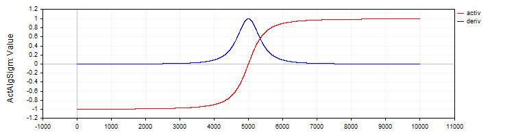
Figure 3. Algebraic sigmoid and its derivative

The C_ActRatSigm class implements a rational sigmoid with activation and derivative methods.

//——————————————————————————————————————————————————————————————————————————————
// Rational sigmoid
class C_ActRatSigm : public C_Base_ActFunc
{
  public:
  C_ActRatSigm () {funcName = "ActRatSigm";}

  double Activ (double x)
  {
    return x / (1.0 + fabs (x));
  }

  double Deriv (double x)
  {
    //1 / (1 + abs (x))^2
    double d = 1.0 + fabs (x);
    return 1.0 / (d * d);
  }
};
//——————————————————————————————————————————————————————————————————————————————

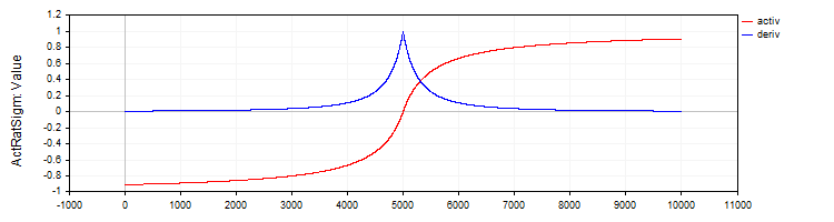
Figure 4. Rational sigmoid and its derivative

The C_ActSoftPlus class implements the Softplus activation function and its derivative.

//——————————————————————————————————————————————————————————————————————————————
// Softplus
class C_ActSoftPlus : public C_Base_ActFunc
{
  public:
  C_ActSoftPlus () {funcName = "ActSoftPlus";}

  double Activ (double x)
  {
    return log (1.0 + exp (x));
  }

  double Deriv (double x)
  {
    return 1.0 / (1.0 + exp (-x));
  }
};
//——————————————————————————————————————————————————————————————————————————————

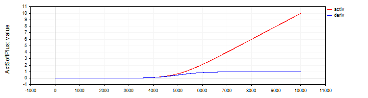
Figure 5. SoftPlus function and its derivative

The C_ActBentIdent class implements the Bent Identity activation function and its derivative.

//——————————————————————————————————————————————————————————————————————————————
// Bent Identity
class C_ActBentIdent : public C_Base_ActFunc
{
  public:
  C_ActBentIdent () {funcName = "ActBentIdent";}

  double Activ (double x)
  {
    return (sqrt (x * x + 1.0) - 1.0) / 2.0 + x;
  }

  double Deriv (double x)
  {
    return x / (2.0 * sqrt (x * x + 1.0)) + 1.0;
  }
};
//——————————————————————————————————————————————————————————————————————————————

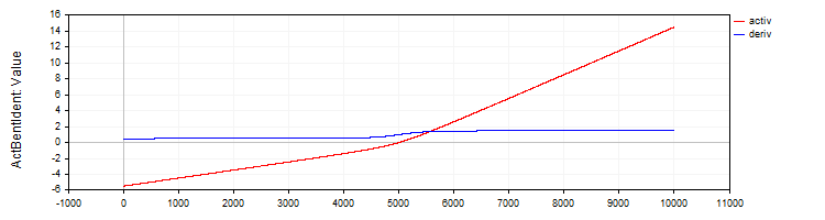
Figure 6. Bent Identity function and its derivative

The C_ActSiLU class provides an implementation of the SiLU activation function and its derivative.

//——————————————————————————————————————————————————————————————————————————————
// SiLU (Swish)
class C_ActSiLU : public C_Base_ActFunc
{
  public:
  C_ActSiLU () {funcName = "ActSiLU";}

  double Activ (double x)
  {
    return x / (1.0 + exp (-x));
  }

  double Deriv (double x)
  {
    if (x == 0.0) return 0.5;

    // f(x) + (f(x)*(1 - f(x)))/ x
    double fx = Activ (x);
    return fx + (fx * (1.0 - fx)) / x;
  }
};
//——————————————————————————————————————————————————————————————————————————————

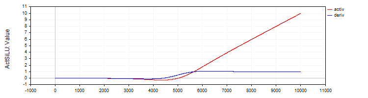
Figure 7. SiLU function and its derivative

The C_ActACON implements the ACON activation function and its derivative.

//——————————————————————————————————————————————————————————————————————————————
// ACON
class C_ActACON : public C_Base_ActFunc
{
  public:
  C_ActACON () {funcName = "ActACON";}

  double Activ (double x)
  {
    return (x * cos (x) + sin (x)) / (1.0 + fabs (x));
  }

  double Deriv (double x)
  {
    if (x == 0.0) return 2.0;

    //[2 * cos(x) - x * sin(x)] / [|x| + 1] - x * (sin(x) + x * cos(x)) / [|x| * ((|x| + 1)²)]
    double sinX   = sin  (x);
    double cosX   = cos  (x);
    double fabsX  = fabs (x);
    double fabsXp = fabsX + 1.0;

    // Divide the equation into two parts
    double part1 = (2.0 * cosX - x * sinX) / fabsXp;
    double part2 = -x * (sinX + x * cosX) / (fabsX * fabsXp * fabsXp);
    return part1 + part2;
  }
};
//——————————————————————————————————————————————————————————————————————————————

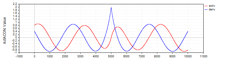
Figure 8. ACON function and its derivative

The C_ActSERF class implements the SERF activation function and its derivative.

//——————————————————————————————————————————————————————————————————————————————
// SERF (sigmoid-weighted exponential straightening function)
class C_ActSERF : public C_Base_ActFunc
{
  public:
  C_ActSERF ()
  {
    alpha    = 0.5;
    funcName = "ActSERF";
  }

  double Activ (double x)
  {
    double sigmoid = 1.0 / (1.0 + exp (-alpha * x));

    if (x >= 0) return sigmoid * x;
    else return sigmoid * (exp (x) - 1.0);
  }

  double Deriv (double x)
  {
    double sigmoid = 1.0 / (1.0 + exp (-alpha * x));
    double sigmoidDeriv = alpha * sigmoid * (1.0 - sigmoid);
    double e = exp (x);
    if (x >= 0) return sigmoid + x * sigmoidDeriv;
    else return sigmoid * e + (e - 1.0) * sigmoidDeriv;
  }

  private:
  double alpha;
};
//——————————————————————————————————————————————————————————————————————————————

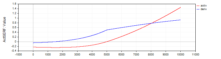
Figure 9. SERF function and its derivative

The C_ActSNAKE class implements the SNAKE activation function and its derivative.

//——————————————————————————————————————————————————————————————————————————————
// Snake (periodic activation function)
class C_ActSnake : public C_Base_ActFunc
{
  public:
  C_ActSnake ()
  {
    frequency = 1;
    funcName  = "ActSnake";
  }

  double Activ (double x)
  {
    double sinx = sin (frequency * x);
    return x + sinx * sinx;
  }

  double Deriv (double x)
  {
    double fx = frequency * x;
    return 1.0 + 2.0 * sin (fx) * cos (fx) * frequency;
  }

  private:
  double frequency;
};
//——————————————————————————————————————————————————————————————————————————————

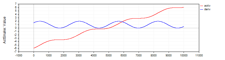
Figure 10. SNAKE function and its derivative

Testing activation functions

Now it is time to look at how an MLP network is trained with different activation functions. The complexity of the activation function for the optimization algorithm can be clearly demonstrated on the 1-1-1 MLP configuration using only one example in training (one input value and one target value).

At first glance, this may not seem obvious. Why does such a simple task spark interest? There is an important methodological point here: using a single data point allows us to isolate and examine the complexity of the activation function itself and its impact on the optimization. When we work with a large dataset, many factors influence training: the distribution of the data, the interdependencies between examples, and how their influence manifests itself when passing through the activation function. By using only one point, we remove all these external factors and can focus on how difficult it is for the optimization algorithm to work with a specific activation function.

The point is that a neural network passing through a single point of the interpolated function can have an infinite number of weight options. This may seem incredible, but it follows from the equation in * w + b = out, where in is a network input, w is a weight, b is a bias, while out is a network output for the configuration 1-1.

There are no problems with this configuration, however, they appear when adding another layer - the 1-1-1 configuration. In this case, even the simplest problem becomes non-trivial for the optimization algorithm, since the search space for a solution becomes significantly more complex: now it is necessary to find the correct combination of weights through the intermediate layer with its activation function. It is this complexity that allows us to evaluate how effectively different optimization algorithms cope with weight tuning when working with different activation functions.

Below are tables with the results of the ADAM algorithms in the classical implementation and the population ADAMm. For both algorithms, 10,000 iterations were performed. For the population-based algorithm, the presence of the population was taken into account, and the total number of neural network calculations remained the same. The printouts indicate the pseudorandom number generator seed (to reproduce problematic training runs), the iteration that yielded the best result, and the result for the current epoch, a multiple of 1000.

The weights were initialized with random numbers using the Xavier method for ADAM and random numbers in the range [-10; 10] for ADAMm. Several tests were performed with different grains and the worst results were selected. The weight selection process was completed either when the maximum number of iterations was reached or when the error decreased below 0.000001.

Table of results for sigmoid activation functions:

Tanh	AlgSigm	RatSigm
MLP config: 1|1|1, Weights: 4, Activation func: eActTanh, Seed: 4 -----Integrated ADAM----- 0: 0.2415125490594974, 0: 0.24151254905949734 0: 0.2415125490594974, 1000: 0.24987227299268625 0: 0.2415125490594974, 2000: 0.24999778562849811 0: 0.2415125490594974, 3000: 0.24999995996010888 0: 0.2415125490594974, 4000: 0.2499999992693791 0: 0.2415125490594974, 5000: 0.24999999998663514 0: 0.2415125490594974, 6000: 0.2499999999997553 0: 0.2415125490594974, 7000: 0.24999999999999556 0: 0.2415125490594974, 8000: 0.25 0: 0.2415125490594974, 9000: 0.25 Best result iteration: 0, Err: 0.241513 -----Population-based ADAMm----- 0: 0.2499999999999871 Best result iteration: 883, Err: 0.000001	MLP config: 1|1|1, Weights: 4, Activation func: eActAlgSigm, Seed: 4 -----Integrated ADAM----- 0: 0.1878131682539310, 0: 0.18781316825393096 0: 0.1878131682539310, 1000: 0.22880505258129305 0: 0.1878131682539310, 2000: 0.2395439537933131 0: 0.1878131682539310, 3000: 0.24376284285887292 0: 0.1878131682539310, 4000: 0.24584964230029535 0: 0.1878131682539310, 5000: 0.2470364071634453 0: 0.1878131682539310, 6000: 0.24777681648987268 0: 0.1878131682539310, 7000: 0.2482702131676117 0: 0.1878131682539310, 8000: 0.24861563983949608 0: 0.1878131682539310, 9000: 0.2488669473265396 Best result iteration: 0, Err: 0.187813 -----Population-based ADAMm----- 0: 0.2481251241755712 1000: 0.0000009070157679 Best result iteration: 1000, Err: 0.000001	MLP config: 1|1|1, Weights: 4, Activation func: eActRatSigm, Seed: 4 -----Integrated ADAM----- 0: 0.0354471509280691, 0: 0.03544715092806905 0: 0.0354471509280691, 1000: 0.10064226929576263 0: 0.0354471509280691, 2000: 0.13866170841306655 0: 0.0354471509280691, 3000: 0.16067944018111643 0: 0.0354471509280691, 4000: 0.17502946224977484 0: 0.0354471509280691, 5000: 0.18520767592761297 0: 0.0354471509280691, 6000: 0.19285431843628092 0: 0.0354471509280691, 7000: 0.1988366186290051 0: 0.0354471509280691, 8000: 0.20365853142896836 0: 0.0354471509280691, 9000: 0.20763502064394074 Best result iteration: 0, Err: 0.035447 -----Population-based ADAMm----- 0: 0.1928944265733889 Best result iteration: 688, Err: 0.000000

Table of results for SiLU type activation functions:

SoftPlus	BentIdent	SiLU
MLP config: 1|1|1, Weights: 4, Activation func: eActSoftPlus, Seed: 2 -----Integrated ADAM----- 0: 0.5380138004155748, 0: 0.5380138004155747 0: 0.5380138004155748, 1000: 131.77685264891647 0: 0.5380138004155748, 2000: 1996.1250363225556 0: 0.5380138004155748, 3000: 8050.259717531171 0: 0.5380138004155748, 4000: 20321.169969814575 0: 0.5380138004155748, 5000: 40601.21872791767 0: 0.5380138004155748, 6000: 70655.44591598355 0: 0.5380138004155748, 7000: 112311.81150857621 0: 0.5380138004155748, 8000: 167489.98562842538 0: 0.5380138004155748, 9000: 238207.27978678182 Best result iteration: 0, Err: 0.538014 -----Population-based ADAMm----- 0: 18.4801637203493884 778: 0.0000022070092175 Best result iteration: 1176, Err: 0.000001	MLP config: 1|1|1, Weights: 4, Activation func: eActBentIdent, Seed: 4 -----Integrated ADAM----- 0: 15.1221330593320857, 0: 15.122133059332086 0: 15.1221330593320857, 1000: 185.646717568436 0: 15.1221330593320857, 2000: 1003.1026112225994 0: 15.1221330593320857, 3000: 2955.8393027057205 0: 15.1221330593320857, 4000: 6429.902382962495 0: 15.1221330593320857, 5000: 11774.781156010686 0: 15.1221330593320857, 6000: 19342.379583340015 0: 15.1221330593320857, 7000: 29501.355075464813 0: 15.1221330593320857, 8000: 42640.534930000824 0: 15.1221330593320857, 9000: 59168.850722337185 Best result iteration: 0, Err: 15.122133 -----Population-based ADAMm----- 0: 7818.0964949082390376 Best result iteration: 15, Err: 0.000001	MLP config: 1|1|1, Weights: 4, Activation func: eActSiLU, Seed: 2 -----Integrated ADAM----- 0: 0.0021199944516222, 0: 0.0021199944516222444 0: 0.0021199944516222, 1000: 4.924850697388685 0: 0.0021199944516222, 2000: 14.827133542234415 0: 0.0021199944516222, 3000: 28.814259008218087 0: 0.0021199944516222, 4000: 45.93517121925276 0: 0.0021199944516222, 5000: 65.82077308420028 0: 0.0021199944516222, 6000: 88.26782602934948 0: 0.0021199944516222, 7000: 113.15535264604428 0: 0.0021199944516222, 8000: 140.41067538093935 0: 0.0021199944516222, 9000: 169.9878269747845 Best result iteration: 0, Err: 0.002120 -----Population-based ADAMm----- 0: 17.2288020548757288 1000: 0.0000030959186317 Best result iteration: 1150, Err: 0.000001

Table of results for periodic activation functions:

ACON	SERF	Snake
MLP config: 1|1|1, Weights: 4, Activation func: eActACON, Seed: 3 -----Integrated ADAM----- 0: 0.8183728267492676, 0: 0.8183728267492675 160: 0.5853150801288914, 1000: 1.2003151947973498 2000: 0.0177702331540612, 2000: 0.017770233154061187 3000: 0.0055801976952827, 3000: 0.005580197695282676 4000: 0.0023096724537356, 4000: 0.002309672453735598 5000: 0.0010238849157595, 5000: 0.0010238849157594616 6000: 0.0004581612824611, 6000: 0.0004581612824611273 7000: 0.0002019092359805, 7000: 0.00020190923598049711 8000: 0.0000867118074097, 8000: 0.00008671180740972474 9000: 0.0000361764073840, 9000: 0.00003617640738397845 Best result iteration: 9999, Err: 0.000015 -----Population-based ADAMm----- 0: 1.3784017183806672 Best result iteration: 481, Err: 0.000000	MLP config: 1|1|1, Weights: 4, Activation func: eActSERF, Seed: 4 -----Integrated ADAM----- 0: 0.2415125490594974, 0: 0.24151254905949734 0: 0.2415125490594974, 1000: 0.24987227299268625 0: 0.2415125490594974, 2000: 0.24999778562849811 0: 0.2415125490594974, 3000: 0.24999995996010888 0: 0.2415125490594974, 4000: 0.2499999992693791 0: 0.2415125490594974, 5000: 0.24999999998663514 0: 0.2415125490594974, 6000: 0.2499999999997553 0: 0.2415125490594974, 7000: 0.24999999999999556 0: 0.2415125490594974, 8000: 0.25 0: 0.2415125490594974, 9000: 0.25 Best result iteration: 0, Err: 0.241513 -----Population-based ADAMm----- 0: 0.2499999999999871 Best result iteration: 883, Err: 0.000001	MLP config: 1|1|1, Weights: 4, Activation func: eActSnake, Seed: 4 -----Integrated ADAM----- 0: 0.2415125490594974, 0: 0.24151254905949734 0: 0.2415125490594974, 1000: 0.24987227299268625 0: 0.2415125490594974, 2000: 0.24999778562849811 0: 0.2415125490594974, 3000: 0.24999995996010888 0: 0.2415125490594974, 4000: 0.2499999992693791 0: 0.2415125490594974, 5000: 0.24999999998663514 0: 0.2415125490594974, 6000: 0.2499999999997553 0: 0.2415125490594974, 7000: 0.24999999999999556 0: 0.2415125490594974, 8000: 0.25 0: 0.2415125490594974, 9000: 0.25 Best result iteration: 0, Err: 0.241513 -----Population-based ADAMm----- 0: 0.2499999999999871 Best result iteration: 883, Err: 0.000001

We can now draw preliminary conclusions about the complexity of activation functions for the classical gradient ADAM and population ADAMm. Although the regular ADAM has direct information about the gradient of the activation function, that is, it literally knows the direction of steepest descent, it failed to cope with such a seemingly simple task. ACON turned out to be the simplest function for ADAM. It is on this type that it was able to consistently minimize the error. But functions like SiLU turned out to be a problem for it: not only did the error not decrease, but it also grew rapidly. It is obvious that since ADAM did not have the weight and bias boundary conditions, it chose the wrong direction and increased the weight values. The weights flew freely to the sides, unrestrained and literally blown away by the directed wind of the activation function derivative.

The problem will only get worse if you use more neurons in layers, because each neuron receives as input the sum of the products of the outputs of the previous layer neurons by the corresponding weight. Thus, the sum can become so large that it becomes impossible to correctly calculate the exponential function.

As we can see, none of the activation functions poses a problem for the population ADAMm. It converges consistently on all of them, and only on some did the number of iterations slightly exceed 1000.

Refining the activation function classes, MLP and ADAM

To correct the situation with scattered weights in the neural network, we will make changes to the activation function classes. This will allow us to track the boundaries of the corresponding functions and prevent the accumulation of a large sum when it is fed to a neuron, and will also limit the values of the weights and biases themselves.

I will add GetBoundUp and GetBoundLo methods to the base class, which provide access to the bounds of the corresponding activation functions, allowing other classes or functions to obtain information about the permissible values.

Below is the code for the base class and the hyperbolic tangent class with some changes made (the rest of the code remains unchanged). The remaining classes of other activation functions are implemented similarly, with their own corresponding boundaries.

//——————————————————————————————————————————————————————————————————————————————
// Base class of the neuron activation function
class C_Base_ActFunc
{
  public:
  double         GetBoundUp  () { return boundUp;}
  double         GetBoundLo  () { return boundLo;}
  protected:
  double boundUp;  // upper bound of the input range
  double boundLo;  // lower bound of the input range
};
//——————————————————————————————————————————————————————————————————————————————

//——————————————————————————————————————————————————————————————————————————————
// Hyperbolic tangent
class C_ActTanh : public C_Base_ActFunc
{
  public:
  C_ActTanh ()
  {
    boundUp  =  6.0;
    boundLo  = -6.0;
  }
};
//——————————————————————————————————————————————————————————————————————————————

Now add validation of the sum values to the MLP forward pass method code before feeding them to the neuron activation function to ensure that they do not go beyond the specified boundaries. There is no point in increasing the sum beyond the specified limits. Moreover, this will allow for an early stop when calculating the sum for a network configuration with a large number of neurons in layers, which can significantly speed up the calculations.

Upper bound check: This code snippet checks if the current value of the sum is greater than the set upper bound. If the value is greater than this bound, it is set equal to this bound and the loop execution is terminated. The lower bound is checked in a similar manner.

//+----------------------------------------------------------------------------+
//| Direct network pass                                                        |
//| Calculate the values of all layers sequentially from input to output       |
//+----------------------------------------------------------------------------+
void C_MLPa::ForwProp (double &inLayer  [],  // input values
                       double &outLayer [])  // output layer values
{
  double val;

  // Set the input layer activation values
  for (int n = 0; n < layersSize [0]; n++)
  {
    nL [0].n [n].out = inLayer [n];
  }

  // Handle hidden and output layers
  for (int ln = 1; ln < nLC; ln++)
  {
    for (int n = 0; n < layersSize [ln]; n++)
    {
      val = nL [ln].n [n].bias;

      for (int w = 0; w < layersSize [ln - 1]; w++)
      {
        val += nL [ln - 1].n [w].out * wL [ln - 1].nOnL [w].nOnR [n].w;

        if (val >  actFunc.GetBoundUp ())
        {
          val =  actFunc.GetBoundUp ();
          break;
        }
        if (val < actFunc.GetBoundLo ())
        {
          val = actFunc.GetBoundLo ();
          break;
        }
      }

      nL [ln].n [n].out = actFunc.Activ (val); // Apply activation function
    }
  }

  // Set the output layer values
  for (int n = 0; n < layersSize [nLC - 1]; n++) outLayer [n] = nL [nLC - 1].n [n].out;
}
//——————————————————————————————————————————————————————————————————————————————

Now let's add the code for verifying the bounds to the backpropagation method. These add-ons implement the logic for reflecting a bias and weight values from given bounds to the inverse bound. It is necessary to ensure that values do not fall outside the acceptable ranges, preventing uncontrolled increases or decreases in weights and biases.

Simply cutting off values at the boundary would lead to stagnation in training, since the weight would simply hit the boundary, and changing the weights would become impossible. It is precisely to prevent such situations that reflection is implemented, rather than value cutting. This provides a "revitalization" or a kind of "shake-up" when adjusting the weights and biases.

//+----------------------------------------------------------------------------+
//| Backward network pass                                                      |
//| Update the weights and biases of all layers from output to input           |
//+----------------------------------------------------------------------------+
void C_MLPa::BackProp (double &errors [])
{
  t++;  // Increase the iteration counter

  double delta;     // current neuron delta
  double deltaNext; // delta of the neuron in the next layer connected to the current neuron
  double out;       // neuron value after applying the activation function
  double deriv;     // derivative
  double w;         // weight for connecting the current neuron to the neuron of the next layer
  double bias;      // bias

  // 1. Calculating deltas for all layers ----------------------------------------
  for (int ln = nLC - 1; ln > 0; ln--)                  // walk through layers in reverse order from output to input
  {
    for (int nCurr = 0; nCurr < layersSize [ln]; nCurr++)        // iterate through the neurons of the current layer
    {
      if (ln == nLC - 1)
      {
        delta = errors [nCurr] * actFunc.Deriv (nL [ln].n [nCurr].out);
      }
      else
      {
        delta = 0.0;

        // Sum the products of the deltas of the next layer by the corresponding weights
        for (int nNext = 0; nNext < layersSize [ln + 1]; nNext++) // pass the neurons of the next layer in the usual order
        {
          deltaNext = nL [ln + 1].n [nNext].delta;
          w         = wL [ln].nOnL [nCurr].nOnR [nNext].w;
          delta    += deltaNext * w;
        }
      }

      // Delta considering the derivative of the sigmoid
      out   = nL [ln].n [nCurr].out;
      deriv = actFunc.Deriv (out);
      nL [ln].n [nCurr].delta = delta * deriv;
    }
  }

  // 2. Update biases using ADAM ------------------------------
  for (int ln = 1; ln < nLC; ln++)
  {
    for (int nCurr = 0; nCurr < layersSize [ln]; nCurr++)
    {
      delta = nL [ln].n [nCurr].delta;

      // Update displacement moments
      nL [ln].n [nCurr].m = beta1 * nL [ln].n [nCurr].m + (1.0 - beta1) * delta;
      nL [ln].n [nCurr].v = beta2 * nL [ln].n [nCurr].v + (1.0 - beta2) * delta * delta;

      // Adjust displacement moments
      double m_hat = nL [ln].n [nCurr].m / (1.0 - pow (beta1, t));
      double v_hat = nL [ln].n [nCurr].v / (1.0 - pow (beta2, t));

      // Update bias
      nL [ln].n [nCurr].bias += alpha * m_hat / (sqrt (v_hat) + epsilon);
      bias = nL [ln].n [nCurr].bias;

      if (bias < actFunc.GetBoundLo ())
      {
        nL [ln].n [nCurr].bias = actFunc.GetBoundUp () - (actFunc.GetBoundLo () - bias);  // reflect from the bottom border 
      }
      else
        if (bias > actFunc.GetBoundUp ())
        {
          nL [ln].n [nCurr].bias = actFunc.GetBoundLo () + (bias - actFunc.GetBoundUp ());  // reflect from the upper border
        }
    }
  }

  // 3. Update weights using ADAM ---------------------------------
  for (int lw = 0; lw < wLC; lw++)
  {
    for (int nCurr = 0; nCurr < layersSize [lw]; nCurr++)
    {
      for (int nNext = 0; nNext < layersSize [lw + 1]; nNext++)
      {
        deltaNext = nL [lw + 1].n [nNext].delta;
        out       = nL [lw].n [nCurr].out;
        double gradient = deltaNext * out;

        // Update moments for weights
        wL [lw].nOnL [nCurr].nOnR [nNext].m = beta1 * wL [lw].nOnL [nCurr].nOnR [nNext].m + (1.0 - beta1) * gradient;
        wL [lw].nOnL [nCurr].nOnR [nNext].v = beta2 * wL [lw].nOnL [nCurr].nOnR [nNext].v + (1.0 - beta2) * gradient * gradient;

        // Adjust weight moments
        double m_hat = wL [lw].nOnL [nCurr].nOnR [nNext].m / (1.0 - pow (beta1, t));
        double v_hat = wL [lw].nOnL [nCurr].nOnR [nNext].v / (1.0 - pow (beta2, t));

        // Update weight
        wL [lw].nOnL [nCurr].nOnR [nNext].w += alpha * m_hat / (sqrt (v_hat) + epsilon);
        w = wL [lw].nOnL [nCurr].nOnR [nNext].w;

        if (w < actFunc.GetBoundLo ())
        {
          wL [lw].nOnL [nCurr].nOnR [nNext].w = actFunc.GetBoundUp () - (actFunc.GetBoundLo () - w);  // reflect from the lower border
        }
        else
          if (w > actFunc.GetBoundUp ())
          {
            wL [lw].nOnL [nCurr].nOnR [nNext].w = actFunc.GetBoundLo () + (w - actFunc.GetBoundUp ());  // reflect from the upper border
          }
      }
    }
  }
}
//——————————————————————————————————————————————————————————————————————————————

Now let's repeat the same tests as above and look at the results obtained. Now there is no explosion of weights, and there is no avalanche-like growth of errors during training.

Table of results for sigmoid activation functions:

Tanh	AlgSigm	RatSigm
MLP config: 1|1|1, Weights: 4, Activation func: eActTanh, Seed: 2 -----Integrated ADAM----- 0: 0.0169277701441132, 0: 0.016927770144113192 0: 0.0169277701441132, 1000: 0.24726166610109795 0: 0.0169277701441132, 2000: 0.24996248252671016 0: 0.0169277701441132, 3000: 0.2499877118017991 0: 0.0169277701441132, 4000: 0.2260068617570163 0: 0.0169277701441132, 5000: 2.2499589217599363 0: 0.0169277701441132, 6000: 2.2499631351033904 0: 0.0169277701441132, 7000: 2.248459789732414 0: 0.0169277701441132, 8000: 2.146138260175548 0: 0.0169277701441132, 9000: 0.15279792149898394 Best result iteration: 0, Err: 0.016928 -----Population-based ADAMm----- 0: 0.2491964938729135 1000: 0.0000010386817829 Best result iteration: 1050, Err: 0.000001	MLP config: 1|1|1, Weights: 4, Activation func: eActAlgSigm, Seed: 2 -----Integrated ADAM----- 0: 0.0095411465043040, 0: 0.009541146504303972 0: 0.0095411465043040, 1000: 0.20977102640908893 0: 0.0095411465043040, 2000: 0.23464558094398064 0: 0.0095411465043040, 3000: 0.23657904914082925 0: 0.0095411465043040, 4000: 0.17812555648593617 0: 0.0095411465043040, 5000: 2.1749975763135927 0: 0.0095411465043040, 6000: 2.2093668968051166 0: 0.0095411465043040, 7000: 2.1657244506071813 0: 0.0095411465043040, 8000: 1.9330415523200173 0: 0.0095411465043040, 9000: 0.10441382194622865 Best result iteration: 0, Err: 0.009541 -----Population-based ADAMm----- 0: 0.2201830630768654 Best result iteration: 750, Err: 0.000001	MLP config: 1|1|1, Weights: 4, Activation func: eActRatSigm, Seed: 1 -----Integrated ADAM----- 0: 1.2866075458561122, 0: 1.2866075458561121 1000: 0.2796061866784148, 1000: 0.2796061866784148 2000: 0.0450819127087337, 2000: 0.04508191270873367 3000: 0.0200306843648248, 3000: 0.020030684364824806 4000: 0.0098744349153286, 4000: 0.009874434915328582 5000: 0.0049448920462547, 5000: 0.00494489204625467 6000: 0.0024344513388710, 6000: 0.00243445133887102 7000: 0.0011602603038120, 7000: 0.0011602603038120354 8000: 0.0005316894732581, 8000: 0.0005316894732581081 9000: 0.0002339388712666, 9000: 0.00023393887126662818 Best result iteration: 9999, Err: 0.000099 -----Population-based ADAMm----- 0: 1.8418367346938778 Best result iteration: 645, Err: 0.000000

Table of results for SiLU type activation functions:

SoftPlus	BentIdent	SiLU
MLP config: 1|1|1, Weights: 4, Activation func: eActSoftPlus, Seed: 2 -----Integrated ADAM----- 0: 0.5380138004155748, 0: 0.5380138004155747 0: 0.5380138004155748, 1000: 12.377378915308087 0: 0.5380138004155748, 2000: 12.377378915308087 3000: 0.1996421769021168, 3000: 0.19964217690211675 4000: 0.1985425345613517, 4000: 0.19854253456135168 5000: 0.1966512639256550, 5000: 0.19665126392565502 6000: 0.1933509943676914, 6000: 0.1933509943676914 7000: 0.1874142582090466, 7000: 0.18741425820904659 8000: 0.1762132792048514, 8000: 0.17621327920485136 9000: 0.1538331138702293, 9000: 0.15383311387022927 Best result iteration: 9999, Err: 0.109364 -----Population-based ADAMm----- 0: 12.3773789153080873 Best result iteration: 677, Err: 0.000001	MLP config: 1|1|1, Weights: 4, Activation func: eActBentIdent, Seed: 4 -----Integrated ADAM----- 0: 15.1221330593320857, 0: 15.122133059332086 0: 15.1221330593320857, 1000: 25.619316876852988 1922: 8.6344718719116980, 2000: 8.634471871911698 1922: 8.6344718719116980, 3000: 8.634471871911698 1922: 8.6344718719116980, 4000: 8.634471871911698 1922: 8.6344718719116980, 5000: 8.634471871911698 1922: 8.6344718719116980, 6000: 8.634471871911698 6652: 4.3033564303197833, 7000: 8.634471871911698 6652: 4.3033564303197833, 8000: 8.634471871911698 6652: 4.3033564303197833, 9000: 7.11489380279475 Best result iteration: 9999, Err: 3.589207 -----Population-based ADAMm----- 0: 25.6193168768529880 Best result iteration: 15, Err: 0.000001	MLP config: 1|1|1, Weights: 4, Activation func: eActSiLU, Seed: 4 -----Integrated ADAM----- 0: 0.6585816582701970, 0: 0.658581658270197 0: 0.6585816582701970, 1000: 5.142928362480306 1393: 0.3271208998291733, 2000: 0.32712089982917325 1393: 0.3271208998291733, 3000: 0.32712089982917325 1393: 0.3271208998291733, 4000: 0.4029355474095988 5000: 0.0114993205601383, 5000: 0.011499320560138332 6000: 0.0003946998191595, 6000: 0.00039469981915948605 7000: 0.0000686308316624, 7000: 0.00006863083166239227 8000: 0.0000176901182322, 8000: 0.000017690118232197302 9000: 0.0000053723044223, 9000: 0.000005372304422295116 Best result iteration: 9999, Err: 0.000002 -----Population-based ADAMm----- 0: 19.9499415647445524 1000: 0.0000057228950379 Best result iteration: 1051, Err: 0.000000

Table of results for periodic activation functions:

ACON	SERF	Snake
MLP config: 1|1|1, Weights: 4, Activation func: eActACON, Seed: 3 -----Integrated ADAM----- 0: 0.8183728267492676, 0: 0.8183728267492675 160: 0.5853150801288914, 1000: 1.2003151947973498 2000: 0.0177702331540612, 2000: 0.017770233154061187 3000: 0.0055801976952827, 3000: 0.005580197695282676 4000: 0.0023096724537356, 4000: 0.002309672453735598 5000: 0.0010238849157595, 5000: 0.0010238849157594616 6000: 0.0004581612824611, 6000: 0.0004581612824611273 7000: 0.0002019092359805, 7000: 0.00020190923598049711 8000: 0.0000867118074097, 8000: 0.00008671180740972474 9000: 0.0000361764073840, 9000: 0.00003617640738397845 Best result iteration: 9999, Err: 0.000015 -----Population-based ADAMm----- 0: 1.3784017183806672 Best result iteration: 300, Err: 0.000000	MLP config: 1|1|1, Weights: 4, Activation func: eActSERF, Seed: 2 -----Integrated ADAM----- 0: 0.0169277701441132, 0: 0.016927770144113192 0: 0.0169277701441132, 1000: 0.24726166610109795 0: 0.0169277701441132, 2000: 0.24996248252671016 0: 0.0169277701441132, 3000: 0.2499877118017991 0: 0.0169277701441132, 4000: 0.2260068617570163 0: 0.0169277701441132, 5000: 2.2499589217599363 0: 0.0169277701441132, 6000: 2.2499631351033904 0: 0.0169277701441132, 7000: 2.248459789732414 0: 0.0169277701441132, 8000: 2.146138260175548 0: 0.0169277701441132, 9000: 0.15279792149898394 Best result iteration: 0, Err: 0.016928 -----Population-based ADAMm----- 0: 0.2491964938729135 1000: 0.0000010386817829 Best result iteration: 1050, Err: 0.000001	MLP config: 1|1|1, Weights: 4, Activation func: eActSnake, Seed: 2 -----Integrated ADAM----- 0: 0.0169277701441132, 0: 0.016927770144113192 0: 0.0169277701441132, 1000: 0.24726166610109795 0: 0.0169277701441132, 2000: 0.24996248252671016 0: 0.0169277701441132, 3000: 0.2499877118017991 0: 0.0169277701441132, 4000: 0.2260068617570163 0: 0.0169277701441132, 5000: 2.2499589217599363 0: 0.0169277701441132, 6000: 2.2499631351033904 0: 0.0169277701441132, 7000: 2.248459789732414 0: 0.0169277701441132, 8000: 2.146138260175548 0: 0.0169277701441132, 9000: 0.15279792149898394 Best result iteration: 0, Err: 0.016928 -----Population-based ADAMm----- 0: 0.2491964938729135 1000: 0.0000010386817829 Best result iteration: 1050, Err: 0.000001

Summary

So, let's summarize our research. Let me remind you of the essence of the experiment: we took two optimization algorithms built on the same logic, but working in fundamentally different ways. The first one (classic ADAM) is a built-in optimizer that operates from within the neural network, with direct access to the activation functions and the entire internal structure — like a navigator with a detailed map of the area. The second one (population ADAMm) is an external optimizer that works with the neural network as a "black box", without any information about its internal structure or the specifics of the task — like a traveler who finds his way by stars and general direction.

We used the same neural network as the object of study for both algorithms. This is critically important because it allows us to localize the source of potential problems: if we encounter difficulties with certain activation functions, we can be confident that this is not a problem with the neural network itself, but with the way the optimization algorithm interacts with these functions.

This experimental setup allows us to clearly see how different activation functions perform in the context of different optimization approaches. It is important to note that we deliberately do not consider the generalization ability of the network or its performance on new data. Our goal is to study the mutual influence of activation functions and optimization algorithms, their compatibility and the efficiency of their interaction.

This approach allows us to get a clear picture of how different optimization strategies perform on different activation functions, without the influence of external factors. The results of the experiment clearly show that sometimes a "blind" external optimizer can be more efficient than an algorithm that has full information about the network structure.

For all activation functions, the external ADAMm showed fast and stable convergence, which suggests that the properties of the activation function do not play a significant role for it. On the other hand, the conventional built-in ADAM encountered serious problems.

Now let's look at the behavior of the built-in ADAM on each of the activation functions and summarize them in the following conclusions:

1. Problematic functions (getting stuck or slow convergence):

• TanH (hyperbolic tangent)
• AlgSigm (algebraic sigmoid)
• SERF (sigmoid-weighted exponential straightening)
• Snake (periodic function)

2. Successful cases (convergence):

• RatSigm (rational sigmoid), the best of the sigmoid functions
  
• SoftPlus
• BentIdent
  
• SiLU (Swish), the best of the second group
  
• ACON (adaptive function), the best of periodic functions
  

3. Patterns:

Classic sigmoid functions (TanH, AlgSigm) exhibit problems with getting stuck. More modern adaptive functions (ACON, SiLU) demonstrate better convergence. Of the periodic functions, ACON shows convergence, while Snake gets stuck.

Thus, the presented study develops a comprehensive approach to neural network optimization that combines weight control, activation function boundaries, and the learning process into a single interconnected system. The key innovation was the introduction of the GetBoundUp and GetBoundLo methods, which allow each activation function to define its own bounds, which are then used to manage the network weights. This mechanism is complemented by a system for early termination of summation when boundaries are reached, which not only prevents redundant computations, especially in large networks, but also ensures control of values before applying the activation function.

A particularly important element was the weight reflection mechanism, which, unlike traditional pruning or normalization, prevents stagnation in learning by "shaking" the weights when they reach their limits. This solution allows the ability to change weights even in critical situations, ensuring the continuity of the training process. The system integration of all these components creates an effective mechanism for preventing weight scattering without losing training flexibility, which is especially important when working with different activation functions. This integrated approach not only solves the problem of weight control but also opens up new perspectives in understanding the interactions of various neural network components during training.

The study does not indicate that ADAM is useless in training neural networks, but rather focuses attention on its response to certain activation functions. Perhaps for large neural networks there is no alternative at all (except for its modern analogues of gradient descent methods). This could be the next topic for considering the efficiency of ADAM (as a representative of modern optimization algorithms using the backpropagation method) in the context of large-scale neural networks, as well as studying the influence of the choice of activation functions on the generalization ability of the network and the stability of its operation on new data.

Programs used in the article

#	Name	Type	Description
1	#C_AO.mqh	Include	Parent class of population optimization algorithms
2	#C_AO_enum.mqh	Include	Enumeration of population optimization algorithms
3	MLPa.mqh	Script	MLP neural network with ADAM
4	Tests and Drawing act func.mq5	Script	Script for visual construction of activation functions
5	Test act func in training.mq5	Script	MLP training script with ADAM and ADAMm