
Reimagining Classic Strategies (Part 17): Modelling Technical Indicators

Applying machine learning and other modern statistical techniques to algorithmic trading is uniquely challenging. The problems faced by our community are exclusive to financial markets — and because of that, they are rarely discussed in broader machine learning circles. As a result, classical supervised learning offers very little practical guidance on issues that matter to our community. One of the most overlooked issues in our field is the fact that, when modeling financial data, we do not have a fixed target. This might not seem problematic at first, but it is.
To illustrate let us think about how these models are applied in medicine — the reader should remember that medicine is the domain from which many supervised learning techniques originally emerged, and our community is "borrowing" these techniques. In medicine, the target variable is definite and well-defined. A doctor might want to classify a patient as either having cancer or not — a binary classification problem with a clear and immutable label. The doctor’s objective never changes, and the target is grounded in physical reality. Moreover, medical models operate within natural constraints — biological, ethical, or procedural — that give the learning problem a consistent structure.
In contrast, the financial domain lacks such structure. As algorithmic traders, we have no fixed definition of the target. We can model the market in terms of annual returns, daily returns, 15-minute returns, annual price appreciation, maximum drawdowns, volatility, or even relative movement between assets. There are, in fact, infinitely many ways to define what the “target” means in a trading context. And although these targets are all derived from the same underlying data, some targets are far more difficult to forecast than others.
This raises a critical question: could our apparent performance ceiling be caused not by model weakness or data quality, but by our poor choice of target? To make matters worse, we do not know in advance what the “right” target is — or whether a universal target even exists across different markets. Each market may have its own optimal formulation of the prediction problem.
From this perspective, it becomes clear that the performance of our statistical models does not necessarily reflect their true capability. The limitations we encounter — the error levels that seem irreducible — are often symptoms of a methodological glass ceiling.
This article will demonstrate that, through careful experimentation and adaptive methodology, we can continually improve our model’s performance simply by rethinking what we are asking the model to predict, not just how we are training it. By cycling through different target definitions, we will show that performance depends not only on data quality and model complexity, but also — and perhaps most importantly — on the methodology through which we frame the learning problem itself.
Fetching Our Data In MetaTrader 5
To begin our exercise, we first fetch the necessary market data from the MetaTrader 5 terminal. For this project, we will be applying several transformations across a large set of features — a total of 22 features will be used throughout this discussion.To ensure consistency between the data our model encounters during training and the data it will receive during live trading, we fetch our data using a dedicated MQL5 script. This approach allows us to reproduce the same data transformations even after the backtesting period.
The script retrieves the four primary price levels — Open, High, Low, and Close — and attaches a technical indicator to each of them. Once these values are obtained, the script records both the raw prices and their corresponding indicator values. Next, we compute the growth (change) for each of the four price levels and their associated indicators. We then calculate the relative growth between each pair of price levels — for example, the growth between Open and High, Open and Low, and Open and Close. This process yields a detailed breakdown of intra-candle price movements, providing the model with a richer understanding of how prices evolve within each bar.
//+------------------------------------------------------------------+
//|                                                    Fetch Data MA |
//|                                      Copyright 2020, CompanyName |
//|                                       http://www.companyname.net |
//+------------------------------------------------------------------+
#property copyright "Copyright 2024, MetaQuotes Ltd."
#property link      "https://www.mql5.com"
#property version   "1.00"
#property script_show_inputs

//--- Define our moving average indicator
#define MA_TYPE   MODE_SMA          //--- Type of moving average we have

//--- Our handlers for our indicators
int ma_handle,ma_o_handle,ma_h_handle,ma_l_handle;

//--- Data structures to store the readings from our indicators
double ma_reading[],ma_o_reading[],ma_h_reading[],ma_l_reading[];

//--- File name
string file_name = Symbol() + " Detailed Market Data As Series Moving Average.csv";

//--- Amount of data requested
input int size = 3000;
input int MA_PERIOD = 5;
input int HORIZON   = 5;

//+------------------------------------------------------------------+
//| Our script execution                                             |
//+------------------------------------------------------------------+
void OnStart()
  {
   int fetch = size + (HORIZON * 2);
//---Setup our technical indicators
   ma_handle   = iMA(_Symbol,PERIOD_CURRENT,MA_PERIOD,0,MA_TYPE,PRICE_CLOSE);
   ma_o_handle = iMA(_Symbol,PERIOD_CURRENT,MA_PERIOD,0,MA_TYPE,PRICE_OPEN);
   ma_h_handle = iMA(_Symbol,PERIOD_CURRENT,MA_PERIOD,0,MA_TYPE,PRICE_HIGH);
   ma_l_handle = iMA(_Symbol,PERIOD_CURRENT,MA_PERIOD,0,MA_TYPE,PRICE_LOW);

//---Set the values as series
   CopyBuffer(ma_handle,0,0,fetch,ma_reading);
   ArraySetAsSeries(ma_reading,true);
   CopyBuffer(ma_o_handle,0,0,fetch,ma_o_reading);
   ArraySetAsSeries(ma_o_reading,true);
   CopyBuffer(ma_h_handle,0,0,fetch,ma_h_reading);
   ArraySetAsSeries(ma_h_reading,true);
   CopyBuffer(ma_l_handle,0,0,fetch,ma_l_reading);
   ArraySetAsSeries(ma_l_reading,true);

//---Write to file
   int file_handle=FileOpen(file_name,FILE_WRITE|FILE_ANSI|FILE_CSV,",");

   for(int i=size;i>=0;i--)
     {
      if(i == size)
        {
         FileWrite(file_handle,"Time",
                   //--- OHLC
                   "True Open",
                   "True High",
                   "True Low",
                   "True Close",
                   //--- MA OHLC
                   "True MA O",
                   "True MA H",
                   "True MA L",
                   "True MA C",
                   //--- Growth in OHLC
                   "Diff Open",
                   "Diff High",
                   "Diff Low",
                   "Diff Close",
                   //--- Growth in MA OHLC
                   "Diff MA Open 2",
                   "Diff MA High 2",
                   "Diff MA Low 2",
                   "Diff MA Close 2",
                   //--- Growth Across Price Levels
                   "O-C",
                   "H-L",
                   "O-H",
                   "O-L",
                   "C-H",
                   "C-L"
                  );
        }

      else
        {
         FileWrite(file_handle,
                   iTime(_Symbol,PERIOD_CURRENT,i),
                   //--- OHLC
                   iOpen(_Symbol,PERIOD_CURRENT,i),
                   iHigh(_Symbol,PERIOD_CURRENT,i),
                   iLow(_Symbol,PERIOD_CURRENT,i),
                   iClose(_Symbol,PERIOD_CURRENT,i),
                   //--- MA OHLC
                   ma_o_reading[i],
                   ma_h_reading[i],
                   ma_l_reading[i],
                   ma_reading[i],
                   //--- Growth in OHLC
                   iOpen(_Symbol,PERIOD_CURRENT,i)   - iOpen(_Symbol,PERIOD_CURRENT,(i + HORIZON)),
                   iHigh(_Symbol,PERIOD_CURRENT,i)   - iHigh(_Symbol,PERIOD_CURRENT,(i + HORIZON)),
                   iLow(_Symbol,PERIOD_CURRENT,i)    - iLow(_Symbol,PERIOD_CURRENT,(i + HORIZON)),
                   iClose(_Symbol,PERIOD_CURRENT,i)  - iClose(_Symbol,PERIOD_CURRENT,(i + HORIZON)),
                   //--- Growth in MA OHLC
                   ma_o_reading[i] - ma_o_reading[(i + HORIZON)],
                   ma_h_reading[i] - ma_h_reading[(i + HORIZON)],
                   ma_l_reading[i] - ma_l_reading[(i + HORIZON)],
                   ma_reading[i] - ma_reading[(i + HORIZON)],
                   //--- Growth Across Price Levels
                   iOpen(_Symbol,PERIOD_CURRENT,i)  - iClose(_Symbol,PERIOD_CURRENT,i),
                   iHigh(_Symbol,PERIOD_CURRENT,i)   - iLow(_Symbol,PERIOD_CURRENT,i),
                   iOpen(_Symbol,PERIOD_CURRENT,i) - iHigh(_Symbol,PERIOD_CURRENT,i),
                   iOpen(_Symbol,PERIOD_CURRENT,i) - iLow(_Symbol,PERIOD_CURRENT,i),
                   iClose(_Symbol,PERIOD_CURRENT,i) - iHigh(_Symbol,PERIOD_CURRENT,i),
                   iClose(_Symbol,PERIOD_CURRENT,i) - iLow(_Symbol,PERIOD_CURRENT,i)
                  );
        }
     }
//--- Close the file
   FileClose(file_handle);
  }
//+------------------------------------------------------------------+

//+------------------------------------------------------------------+
//| Undefine system constants                                        |
//+------------------------------------------------------------------+
#undef MA_TYPE
//+------------------------------------------------------------------+
Getting Started With Our Analysis in Python
Once the script for data extraction is complete, we move into Python for analysis. As with most of our machine learning experiments, our first goal is to establish a baseline performance level using classical modeling paradigms. We begin by loading our standard Python libraries.
#Import the libraries we need to get started
import pandas as pd
import numpy as np
import matplotlib.pyplot as plt
import seaborn as sns
It is worth noting that the initial version of our MQL5 script used here differs slightly from the final version presented later in this discussion — the earlier version retrieves 17 columns, whereas the final version includes additional features. These discrepancies, and the motivation for expanding the dataset, will become clear by the end of the article.
#Read in the data
data = pd.read_csv("../EURUSD Detailed Market Data As Series Moving Average.csv")
data
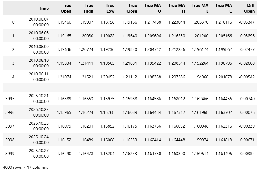
Figure 1: Our dataset is quite large and contains 17 columns in its initial state
After reading in the dataset, we now proceed to label our data using the classical one-step-ahead approach.
#Classical Target
#Baseline value
HORIZON = 1

#Label the data
data['Target'] = data['True Close'].shift(-HORIZON)

#Drop the last batch of forecasts
data = data.iloc[:-HORIZON,:]
data
Readers should recall that we intend to evaluate this statistical model by backtesting it. Therefore, we will drop the last three years of observations and keep them in a separate test set. We will not fit the model on this test set because that would defeat the purpose of our discussion.
#Drop the last 3 years of data
test = data.iloc[-(365*3):,:]
data = data.iloc[:-(365*3),:]
It is interesting to notice that the strength of correlation between the target and the inputs is particularly unstable over time. We examined this by calculating the Pearson correlation between our target and each input variable using an expanding window of observations. This gives us a vector whose values represent the strength of correlation between the target and each input. We then took the L1 norm (the sum of absolute values) of this vector to obtain a single measure of total correlation strength.
We began with one day of data, then two days, three days, and so on, expanding gradually until we reached a full year (365 days). As shown in the figure below, the level of correlation is not stationary — it fluctuates. On some days, it appears strong; on others, it weakens. Overall, it seems to decay as the window expands, suggesting that the relationships between inputs and the target are unstable over time.
corr_strength = []
EPOCHS = 365

for i in np.arange(EPOCHS):
    corr_strength.append(np.linalg.norm(data.loc[:i+1,:].corr().iloc[:,-1],ord=1))


sns.barplot(corr_strength)
plt.ylabel('Correlational Strength')
plt.title('Correlation Between Future Price And Historical Data')
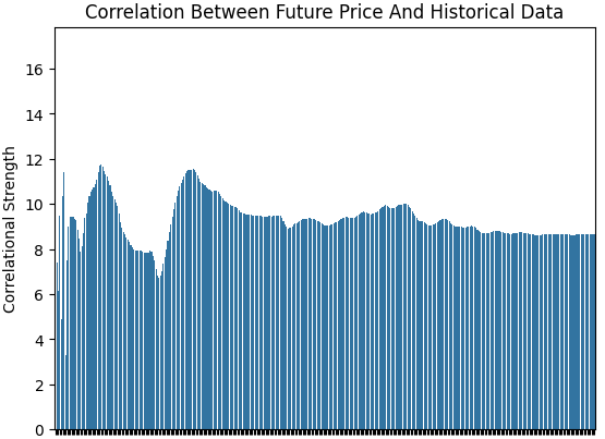
Figure 2: The strength of correlation across the historical EURUSD dataset is not stationary
Next, we visualized the correlational structure among all inputs across the training set using a heatmap. As we can see, the target tends to have strong correlation with the real-valued price levels and their moving averages, while the changes in those inputs are only weakly correlated with the target.
sns.heatmap(data.iloc[:,1:].corr())
plt.title('Analyzing Market Correlation Strucute') 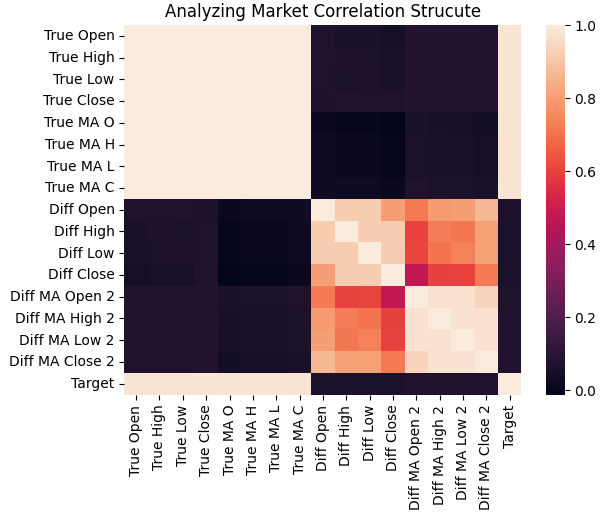
Figure 3: The correlational structure of our historical EURUSD market data shows that the target is strongly related to historical prices
That is not all we can learn from the correlation matrix. We can also perform eigen decomposition on it using the eig function in NumPy, which returns both the eigenvalues and eigenvectors. For now, we focus on the eigenvalues. Eigen values reveal how much variance in the correlation structure is captured by each principal component. In other words, eigenvalues tell us how many dominant “modes of expression” our market data appears to have.
A stable market is typically governed by one dominant mode — such as a strong trend or a mean-reverting process — while a more chaotic market exhibits several competing modes. In our case, the bar plot of eigenvalues shows two large, dominant modes and a third slightly above the average threshold. This suggests that our system may have two dominant modes of behavior and a weaker third one. The remaining eigenvalues are negligible and can be ignored because they do not contribute meaningfully to the correlational structure of the data.
eig_val ,eig_vec =np.linalg.eigh(data.iloc[:,1:].corr())
sns.barplot(eig_val,color='black')
plt.axhline(np.mean(eig_val),color='red',linestyle=':')
plt.ylabel('Eigen Value')
plt.title('Spectrum Analysis of The EURUSD Market')
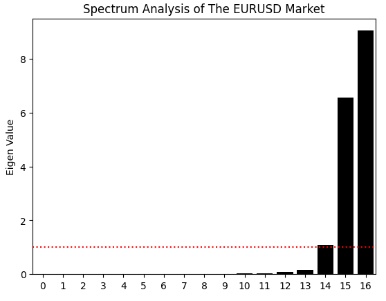
Figure 4: The eigen values of the correlational structure of our historical EURUSD data suggests that the market has 3 major unstable modes
We now proceed to load our statistical learning libraries
from sklearn.linear_model import LinearRegression
Define our inputs and target. We will start off with a simple model that takes 4 inputs.
X = ['True Open','True High','True Low','True Close']
y = 'Target'
Fit the model on our market data.
model = LinearRegression()

model.fit(data.loc[:,X],data[y])
The model appears to have a reasonable grasp of market outcomes even out of sample.
preds = model.predict(test.loc[:,X])

plt.plot(preds,color='black')
plt.plot(test.loc[:,y].values,color='red',linestyle=':')
plt.title('Visualizing Our Accuracy Out of Sample')
plt.xlabel('Historical Time')
plt.ylabel('EURUSD Exchange Rate')
plt.legend(['Model Predictions','Observed Exchange Rate'])
plt.grid()
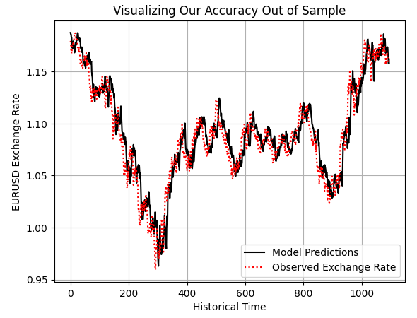
Figure 5: Exploring our model's out of sample predictions to test if the model is sound
Exporting To ONNX
We are now ready to export our learned statistical model to ONNX format. ONNX, which stands for Open Neural Network Exchange, is a globally recognized API that allows developers to build and deploy machine learning models without carrying over any dependencies from the training framework used to create them. To get started, we load the necessary ONNX libraries.
import onnx
from skl2onnx import convert_sklearn
from skl2onnx.common.data_types import FloatTensorType
Next, we define the input and output shapes of our model. In our case, the model takes four inputs and produces one output.
initial_types = [('float_input',FloatTensorType([1,4]))]
final_types = [('float_output',FloatTensorType([1,1]))]
From here, we create an ONNX protocol buffer — an intermediary structure that holds our model before the final conversion.
onnx_proto = convert_sklearn(model,initial_types=initial_types,final_types=final_types,target_opset=12) Once this is done, we save the model as a .onnx file by passing both the ONNX protobuf and the desired filename to the ONNX save function.
onnx.save(onnx_proto,"EURUSD 2022-2025 LR.onnx") Establishing A Baseline Using Classical Techniques
With that complete, we are ready to begin building our trading application in MQL5. The first step is to import the ONNX file that we just exported from our Python analysis.
//+------------------------------------------------------------------+
//|                                                    Benchmark.mq5 |
//|                                               Gamuchirai Ndawana |
//|                    https://www.mql5.com/en/users/gamuchiraindawa |
//+------------------------------------------------------------------+
#property copyright "Gamuchirai Ndawana"
#property link      "https://www.mql5.com/en/users/gamuchiraindawa"
#property version   "1.00"

//+------------------------------------------------------------------+
//| System resources                                                 |
//+------------------------------------------------------------------+
#resource "\\Files\\EURUSD 2022-2025 LR.onnx" as const uchar onnx_proto[];
We then load several supporting libraries that will help us perform routine tasks, such as opening, closing, and modifying trades, checking for new candles, managing ONNX buffers, and other related operations.
//+------------------------------------------------------------------+
//| Libraries                                                        |
//+------------------------------------------------------------------+
#include <Trade\Trade.mqh>
#include <VolatilityDoctor\Time\Time.mqh>
#include <VolatilityDoctor\ONNX\ONNXFloat.mqh>
#include <VolatilityDoctor\Trade\TradeInfo.mqh>

CTrade    Trade;
Time      *time;
TradeInfo *trade;
ONNXFloat *onnx_model;
Next, we initialize a few global variables that will be used throughout the application.
//+------------------------------------------------------------------+
//| Global variables                                                 |
//+------------------------------------------------------------------+
int atr_handler;
double atr[];
float prediction;
During initialization, we create our ONNX model from the buffer we loaded earlier. In previous discussions, we developed a dedicated library to handle ONNX files efficiently. Thanks to this custom library, the number of setup steps required to load and use our ONNX model has been greatly reduced.
//+------------------------------------------------------------------+
//| Expert initialization function                                   |
//+------------------------------------------------------------------+
int OnInit()
  {
//---
   onnx_model = new ONNXFloat(onnx_proto);
   trade      = new TradeInfo(Symbol(),PERIOD_CURRENT);
   time       = new Time(Symbol(),PERIOD_D1);
   atr_handler = iATR(Symbol(),PERIOD_CURRENT,14);

   if(!onnx_model.DefineOnnxInputShape(0,1,4))
     {
      Print("Failed to specify ONNX input shape");
      return(INIT_FAILED);
     }

   if(!onnx_model.DefineOnnxOutputShape(0,1,1))
     {
      Print("Failed to specify ONNX output shape");
      return(INIT_FAILED);
     }

//---
   return(INIT_SUCCEEDED);
  }
When we are no longer using the ONNX model or other allocated resources, we ensure to free them properly, as this is considered best practice in MetaTrader 5 development.
//+------------------------------------------------------------------+
//| Expert deinitialization function                                 |
//+------------------------------------------------------------------+
void OnDeinit(const int reason)
  {
//---
   delete onnx_model;
   delete time;
   delete trade;
  }
Whenever new price data arrives, we update our indicator buffers, define the appropriate input values for the ONNX model, and retrieve a prediction. Based on the prediction, we execute or close trades accordingly. If any issue occurs, an error message is displayed to the user.
//+------------------------------------------------------------------+
//| Expert tick function                                             |
//+------------------------------------------------------------------+
void OnTick()
  {
//---
   if(time.NewCandle())
     {
      if(PositionsTotal()==0)
        {
         CopyBuffer(atr_handler,0,0,1,atr);
         onnx_model.DefineInputValues(0,(float) iOpen(Symbol(),PERIOD_CURRENT,0));
         onnx_model.DefineInputValues(1,(float) iHigh(Symbol(),PERIOD_CURRENT,0));
         onnx_model.DefineInputValues(2,(float) iLow(Symbol(),PERIOD_CURRENT,0));
         onnx_model.DefineInputValues(3,(float) iClose(Symbol(),PERIOD_CURRENT,0));
         double padding = (atr[0]*1.5);

         if(onnx_model.Predict())
           {
            prediction = onnx_model.GetPrediction(0);
            Print("Onnx Prediction:\n",prediction);

            if(prediction > iClose(Symbol(),PERIOD_CURRENT,0))
              {
               Trade.Buy(trade.MinVolume(),Symbol(),trade.GetAsk(),trade.GetBid()-padding,trade.GetBid()+padding,"");
              }

            if(prediction < iClose(Symbol(),PERIOD_CURRENT,0))
              {
               Trade.Sell(trade.MinVolume(),Symbol(),trade.GetBid(),trade.GetAsk()+padding,trade.GetAsk()-padding,"");
              }
           }
         else
           {
            Print("Failed to obtain a prediction from our model: ",GetLastError());
            return;
           }
        }
     }
  }
//+------------------------------------------------------------------+
At this point, we are ready to begin our backtest. We start by selecting the application we want to test — in this case, the benchmark version of our trading system. We define the testing period, which spans from 2022 up to October 2025 (the time of writing).

Figure 6: The initial baseline backtest is very important, it gives us a benchmark to aim for
We then specify the testing conditions under which the strategy should be evaluated. To simulate realistic market behavior, we enable random delay, which helps approximate the unpredictable nature of live trading.
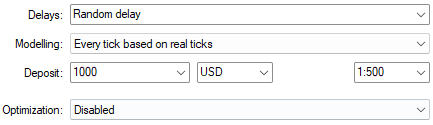
Figure 7: Select random delay settings for a realistic emulation of real time market conditions
As we can see from the results, the strategy appears rather unstable under this simple setup. These results are not entirely surprising, since the model is designed to predict only one step ahead — effectively making trade-by-trade, candle-by-candle predictions. This approach is not how a human trader views the market, and it naturally limits the system’s realism and robustness. Nevertheless, this serves as our baseline result, derived by following standard best practices.
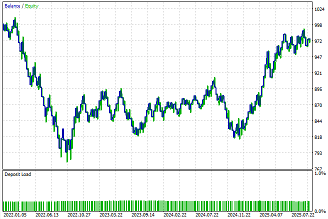
Figure 8: The equity curve produced by the first version of our trading application calls us to apply more effort
Upon closer examination of the backtest, we observe that the system is severely underperforming. Not only does it consistently lose money throughout the backtest, but its trade distribution is also suboptimal and reflects no meaningful understanding of market dynamics. Over a three-year window, the statistical model opened 183 long trades and only one short trade. This imbalance highlights the model’s inability to interpret the market effectively — and clearly demonstrates that we can achieve far better performance than what standard machine learning practices alone might suggest.

Figure 9: The detailed statistics of our trading application reveal flaws in the traditional approach
Improving The Baseline Using Classical Tecniques
Let us now begin implementing improvements to our trading application. The first enhancement we can make concerns our forecasting horizon. Generally speaking, forecasting only one step into the future does not reflect how profitable human traders operate. Therefore, we will extend our forecast horizon to 10 steps ahead, which should provide a more realistic outlook than a single-step prediction. At this stage, the rest of the code within our Jupyter notebook remains unchanged, so we have omitted those sections and will only highlight the segments that differ.
#Classical Target
#V1 value
HORIZON = 10
After fitting our model to look 10 steps ahead, we save it to file and then load the updated version into our trading application.
onnx.save(onnx_proto,"EURUSD 2022-2025 LR V1.onnx") Implementing The Improvements to Our MetaTrader 5 Application
As mentioned earlier, the overall structure of the application remains largely the same. Hence, we exclude unchanged code segments for brevity.
//+------------------------------------------------------------------+
//| System resources                                                 |
//+------------------------------------------------------------------+
#resource "\\Files\\EURUSD 2022-2025 LR V1.onnx" as const uchar onnx_proto[];
Once the updated model has been embedded into the application, we proceed to run a new backtest over the same period to evaluate its performance.
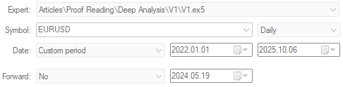
Figure 10: We will now evaluate our first attempt to outperform the benchmark version of our trading application
When examining the equity curve produced by this new version of our system, we observe that very little has changed visually between the two versions. However, a closer look at the detailed statistics reveals a few meaningful improvements.
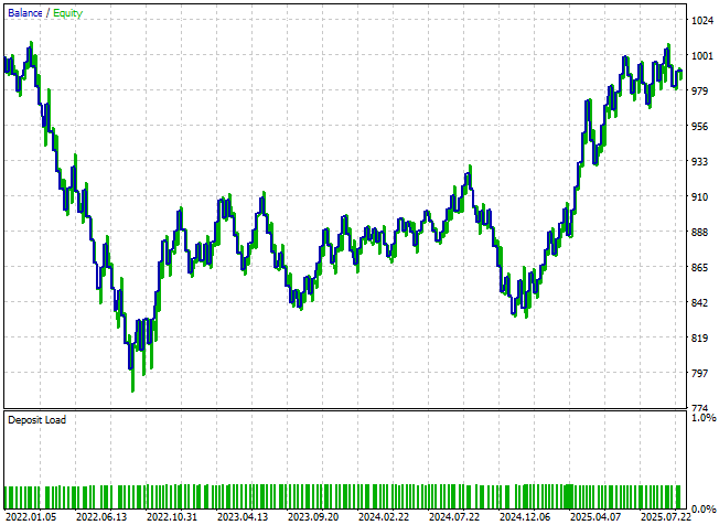
Figure 11: The equity curve produced by our first attempt at improving our trading application appears identical to the first application we started with
The total net loss has decreased significantly—from −$24 to −$8—though the result is still undesirable. Moreover, the total number of short trades remains at zero, indicating that the system still lacks a balanced or comprehensive understanding of market direction. It is therefore clear that, while the modifications have helped, there is still substantial room for improvement.
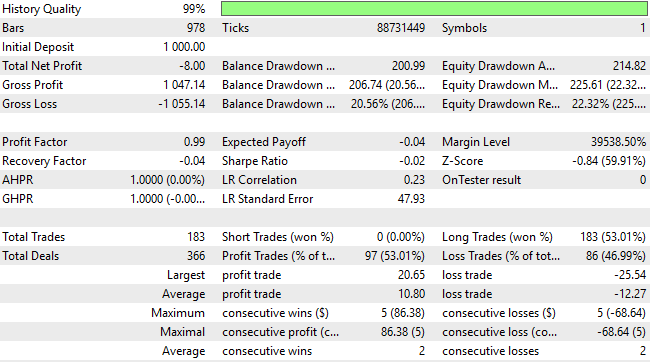
Figure 12: A detailed analysis of our new results indicate that we have made some improvements, but we are still a long way from where we want to be
Outperforming The Classical Techniques
At this point, we have nearly exhausted the principles of classical modeling. Therefore, we will now begin to break away from traditional ideologies and seek improvements based on the insights gathered throughout this series of articles. One particularly meaningful observation we’ve made is that, in most markets, technical indicators often appear easier to forecast than the raw price itself. Building on that insight, we will now modify our modeling setup by changing the target variable—from the future value of price to the future value of the moving average.#Classical Target #V1 value HORIZON = 10 #Label the data data['Target'] = data['True MA C'].shift(-HORIZON) #Drop the last batch of forecasts data = data.iloc[:-HORIZON,:] data
Naturally, this change requires us to redefine our model’s input space as well. We will introduce four new variables describing the current state of the moving averages, expanding our total feature set.
X = ['True Open','True High','True Low','True Close','True MA O','True MA H','True MA L','True MA C']
y = 'Target'
Consequently, we must also revise the input shape of our model to reflect this updated configuration.
initial_types = [('float_input',FloatTensorType([1,8]))]
final_types = [('float_output',FloatTensorType([1,1]))]
Once complete, we save the new model.
onnx.save(onnx_proto,"EURUSD 2022-2025 R V2.onnx") Implementing Our Improvements in MQL5
Now we update our trading application to reference the updated ONNX model.
//+------------------------------------------------------------------+
//|                                                    Benchmark.mq5 |
//|                                               Gamuchirai Ndawana |
//|                    https://www.mql5.com/en/users/gamuchiraindawa |
//+------------------------------------------------------------------+
#property copyright "Gamuchirai Ndawana"
#property link      "https://www.mql5.com/en/users/gamuchiraindawa"
#property version   "1.00"


//+------------------------------------------------------------------+
//| System resources                                                 |
//+------------------------------------------------------------------+
#resource "\\Files\\EURUSD 2022-2025 R V2.onnx" as const uchar onnx_proto[];
Since the moving average indicators are now part of the model’s input space, we begin by defining system constants that specify both the period and type of moving averages being used.
//--- System constants
#define MA_PERIOD 5
#define MA_TYPE MODE_SMA
We then create indicator handles to continuously read and update the latest moving average values as new price levels arrive.
//---Setup our technical indicators
   atr_handler = iATR(Symbol(),PERIOD_CURRENT,14);
   ma_handle   = iMA(_Symbol,PERIOD_CURRENT,MA_PERIOD,0,MA_TYPE,PRICE_CLOSE);
   ma_o_handle = iMA(_Symbol,PERIOD_CURRENT,MA_PERIOD,0,MA_TYPE,PRICE_OPEN);
   ma_h_handle = iMA(_Symbol,PERIOD_CURRENT,MA_PERIOD,0,MA_TYPE,PRICE_HIGH);
   ma_l_handle = iMA(_Symbol,PERIOD_CURRENT,MA_PERIOD,0,MA_TYPE,PRICE_LOW);
Our procedure for opening trades also changes. First, we copy the latest indicator values from the four moving average handles into their respective buffers. Then, using a function from our OnyxTools library called DefineInputValues(), we prepare the current inputs for the ONNX model. Afterward, we call the OnyxPredict() function to obtain a prediction, which is stored in a floating-point variable named prediction. Once the forecast is obtained, we compare the model’s predicted future value of the moving average against its current value. If the moving average is expected to rise, we open long positions. If it is expected to fall, we open short positions.
//+------------------------------------------------------------------+
//| Expert tick function                                             |
//+------------------------------------------------------------------+
void OnTick()
  {
//---
   if(time.NewCandle())
     {
      if(PositionsTotal()==0)
        {
         CopyBuffer(atr_handler,0,0,1,atr);
         CopyBuffer(ma_handle,0,0,1,ma_reading);
         CopyBuffer(ma_o_handle,0,0,1,ma_o_reading);
         CopyBuffer(ma_h_handle,0,0,1,ma_h_reading);
         CopyBuffer(ma_l_handle,0,0,1,ma_l_reading);

         onnx_model.DefineInputValues(0,(float) iOpen(Symbol(),PERIOD_CURRENT,0));
         onnx_model.DefineInputValues(1,(float) iHigh(Symbol(),PERIOD_CURRENT,0));
         onnx_model.DefineInputValues(2,(float) iLow(Symbol(),PERIOD_CURRENT,0));
         onnx_model.DefineInputValues(3,(float) iClose(Symbol(),PERIOD_CURRENT,0));
         onnx_model.DefineInputValues(4,(float) ma_o_reading[0]);
         onnx_model.DefineInputValues(5,(float) ma_h_reading[0]);
         onnx_model.DefineInputValues(6,(float) ma_l_reading[0]);
         onnx_model.DefineInputValues(7,(float) ma_reading[0]);

         double padding = (atr[0]*1.5);

         if(onnx_model.Predict())
           {
            prediction = onnx_model.GetPrediction(0);
            Print("Onnx Prediction:\n",prediction);

            if(ma_reading[0]>ma_o_reading[0])
              {
               if(prediction > ma_reading[0])
                 {
                  Trade.Buy(trade.MinVolume(),Symbol(),trade.GetAsk(),trade.GetBid()-padding,trade.GetBid()+padding,"");
                 }
              }

            if(ma_reading[0]<ma_o_reading[0])
              {
               if(prediction < ma_reading[0])
                 {
                  Trade.Sell(trade.MinVolume(),Symbol(),trade.GetBid(),trade.GetAsk()+padding,trade.GetAsk()-padding,"");
                 }
              }
           }
         else
           {
            Print("Failed to obtain a prediction from our model: ",GetLastError());
            return;
           }
        }
     }
  }
//+------------------------------------------------------------------+
As before, we run this new version of the application over the same test period, which the model has never seen during training.

Figure 13: Running our revised trading application over the same back test window to evaluate our improvements
The equity curve now finally begins to show signs of health—forming an upward trend, though it still exhibits some volatility.
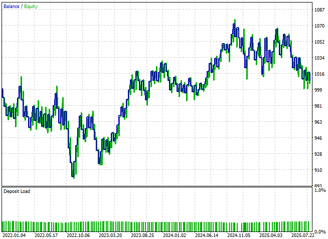
Figure 14: Our application has finally broken past the break-even level for the first time
When we review the detailed performance statistics, we find that the strategy has broken past breakeven. While profits remain modest, the proportion of profitable trades has risen above 50%, settling around 53%, and the profit factor now indicates positive expectancy. Clearly, these refinements are pushing the system in the right direction—though there is still more room for improvement.
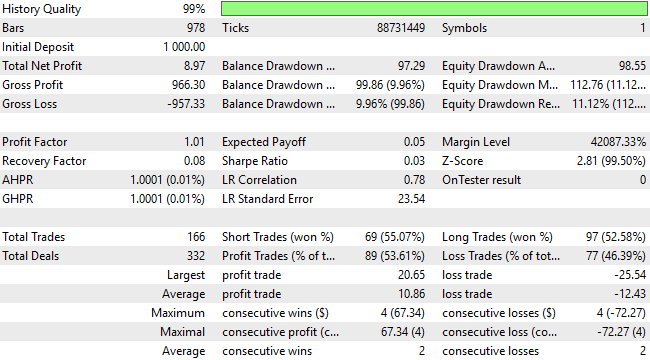
Figure 15: The application appears to have a balanced view of short and long entries, although its profitability is unnaceptable
Realizing More Room For Improvement
As we continue to move away from classical ideologies, we can draw upon another key observation from our related series of articles, Overcoming the Limitations of AI. In that study, we observed that using multiple forecast horizons can sometimes produce models that are more internally coherent—that is, more consistent with themselves—than they are with the real-world data. We will now test whether that same insight can help us in this exercise. To do so, we will create two targets for our model.
Namelyly, the value of the moving average indicator one step ahead, and the value of the same indicator ten steps ahead. For readers who have not read the earlier article, the logic behind this approach is straightforward: we will take our trading signals from the implied slope between the two prediction horizons. In other words— if the moving average is expected to fall across the two forecast horizons, we will sell. Otherwise, if it is expected to rise, we will buy.
#Classical Target
#V1 value
HORIZON = 10

#Label the data
data['Target 1'] = data['True MA C'].shift(-1)
data['Target 2'] = data['True MA C'].shift(-HORIZON)

#Drop the last batch of forecasts
data = data.iloc[:-HORIZON,:]
data
As expected, these changes will alter the output shape of our ONNX model. Therefore, we must update the model definition to reflect the new output configuration.
initial_types = [('float_input',FloatTensorType([1,8]))]
final_types = [('float_output',FloatTensorType([1,2]))]
Then save and reload the revised model within our application.
onnx.save(onnx_proto,"EURUSD 2022-2025 R MFH V3.onnx") Implementing The Improvements In MQL5
Now we load the updated ONNX file.//+------------------------------------------------------------------+ //| System resources | //+------------------------------------------------------------------+ #resource "\\Files\\EURUSD 2022-2025 R MFH V3.onnx" as const uchar onnx_proto[];
Once loaded, we define the new model shape.
   if(!onnx_model.DefineOnnxOutputShape(0,2,1))
     {
      Print("Failed to specify ONNX output shape");
      return(INIT_FAILED);
     }
Now we make all necessary adjustments to how predictions are interpreted. It is important to emphasize that, at this stage, we are no longer comparing the model’s predictions against the real value of the indicator. Instead, we are trading purely on the implied slope between the short- and long-term forecasts.
if(onnx_model.Predict())
           {
            onnx_model.GetPrediction(0);
            Print("Onnx Prediction:\n",prediction);

            if(ma_reading[0]>ma_o_reading[0])
              {
               if(onnx_model.GetPrediction(1)  >  onnx_model.GetPrediction(0))
                 {
                  Trade.Buy(trade.MinVolume(),Symbol(),trade.GetAsk(),trade.GetBid()-padding,trade.GetBid()+padding,"");
                 }
              }

            if(ma_reading[0]<ma_o_reading[0])
              {
               if(onnx_model.GetPrediction(1) <  onnx_model.GetPrediction(0))
                 {
                  Trade.Sell(trade.MinVolume(),Symbol(),trade.GetBid(),trade.GetAsk()+padding,trade.GetAsk()-padding,"");
                 }
              }
           }
For those following along in practice, I recommend maintaining a clear file hierarchy. On my local workstation, I created a separate folder for each version of the application. This helps maintain good working standards and makes it easy to roll back to earlier versions whenever needed.
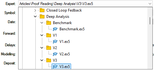
Figure 16: Maintaining a clear file structure is important when making iterative improvements to an applicaiton
Once the appropriate version of the application is ready, we run our tests over the same backtest window as before.
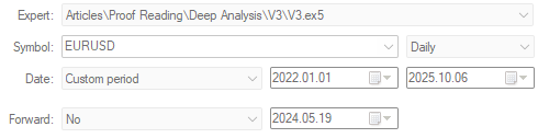
Figure 17: Backtesting the third version of our application over the test period to evaluate the changes we have made
The resulting equity curve reveals an outstanding improvement compared to our initial results. The upward trend is now much more pronounced and dominant than when we first began this analysis. Moreover, the application now breaks into new equity highs that were previously unattainable when forecasting future price levels directly. Although some volatility remains in the balance curve and full stabilization has not yet been achieved, the overall growth trajectory is clearly stronger.
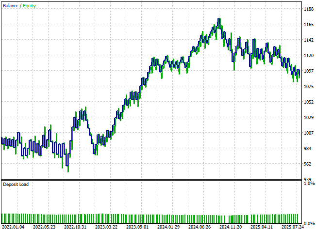
Figure 18: Our new equity curve demonstrates that our application is now reaching new highs we were not able to reach prior.
When we review the detailed results, we see material improvements: the system has moved from an initial loss of 24 units to a profit of 90 units—a remarkable transformation. This is especially impressive given that we have not increased the strategy’s complexity nor changed the modeling architecture. Every gain achieved thus far comes purely from identifying better methodological choices and discarding those that no longer serve our goals.
A closer look at trade distribution reveals further insight. The updated version of the application now executes significantly more short trades, correcting one of the major weaknesses of the earlier version, which struggled to identify selling opportunities. The model now classifies short trades with about 62% accuracy, though it remains slightly biased—placing roughly twice as many long positions as short ones. This calls us to greater effort by asking the question: while performance has improved considerably, is there still yet more room for further refinement?
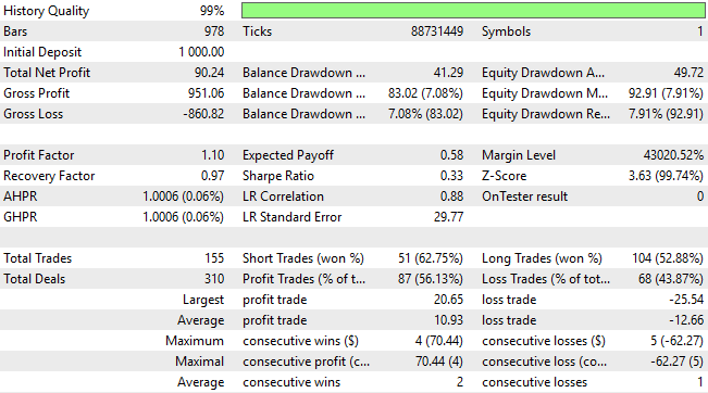
Figure 19: A detailed analysis of the results we obtained from the third version of our trading application
Searching For Further Refinements
We are now ready to dig deeper for further improvements to our trading application. After time for reflection, I considered that we might achieve better results by giving our model a more detailed description of the current market state. To accomplish this, I introduced several new features into our dataset, bringing the total to 23 input variables. All 23 features are fully captured by the scripts provided at the beginning of this article.
#Read in the data
data = pd.read_csv("../EURUSD Detailed Market Data As Series Moving Average.csv")
data
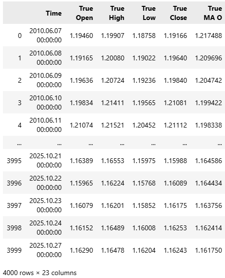
Figure 20: Our updated market data has 23 columns in total
With these additions, we can now examine how the correlational structure of the data has changed. When comparing the new heatmap to the earlier one shown in Figure 3, the differences are striking. This time, if we focus on the two forecast targets, we can observe a much more reliable and structured correlation pattern between the targets and the inputs. Unlike in Figure 3—where the target variables showed weak or inconsistent relationships with the inputs—the new heatmap is clearly hotter, indicating stronger and more meaningful dependencies within the data.
This improvement makes sense. As the reader may recall, the moving average values we are now forecasting are directly derived from price levels. Therefore, a strong correlation between the moving averages and the inputs is both expected and desirable, since the moving average is essentially a weighted sum of past prices.
sns.heatmap(data.iloc[:,1:].corr())
plt.title('Analyzing Market Correlation Strucute') 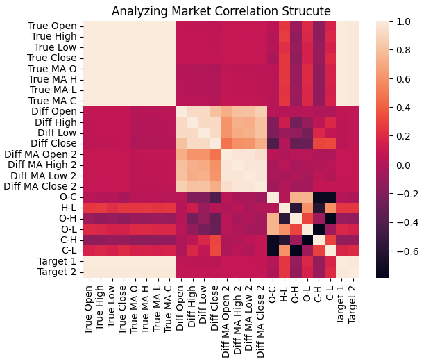
Figure 21: Our updated market data exhibits stronger correlation levels than what we started with in Figure 3
However, when we analyze the spectrum of eigenvalues produced from the correlation matrix of this new dataset, a more complex picture emerges. In Figure 4, representing the earlier dataset, we observed roughly two dominant eigenvalues, with a third only slightly above average. This meant the system previously had two strong modes of expression, and a third that was relatively minor.
Now, in the updated representation of the market—after adding the new features—we find four eigenvalues above the average threshold. This is a critical observation. It suggests that our enriched feature set has introduced additional dominant modes of expression, or in simpler terms, more distinct market regimes.While this provides a richer description of the market, it also introduces a challenge: the data now expresses a higher degree of structural complexity, which can make reliable modeling more difficult. The system we are trying to model now exhibits more regimes and dynamic behaviors than before.
eig_val ,eig_vec =np.linalg.eigh(data.iloc[:,1:].corr())
sns.barplot(eig_val,color='black')
plt.axhline(np.mean(eig_val),color='red',linestyle=':')
plt.ylabel('Eigen Value')
plt.title('Spectrum Analysis of The EURUSD Market')
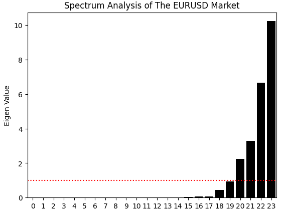
Figure 22: Unfortunately, the market data also appears to be growing more complex with competing modes of expression
Nevertheless, we proceed by separating our input variables from the target variables.
X = data.iloc[:,1:-2].columns
y = ['Target 1','Target 2']
Definine the updated input shape for the model.
initial_types = [('float_input',FloatTensorType([1,len(X)]))]
final_types = [('float_output',FloatTensorType([1,2]))]
Finally, save the newly trained model to file.
onnx.save(onnx_proto,"EURUSD 2022-2025 R V4.onnx") For readers curious about the precise configuration—the new model now has 22 input features.
len(X)
22
Implementing Our Improvements
Once the model is trained, we load it into our trading application.
//+------------------------------------------------------------------+
//| System resources                                                 |
//+------------------------------------------------------------------+
#resource "\\Files\\EURUSD 2022-2025 R V4.onnx" as const uchar onnx_proto[];
And remember to update the ONNX model definition accordingly.
   if(!onnx_model.DefineOnnxInputShape(0,1,22))
     {
      Print("Failed to specify ONNX input shape");
      return(INIT_FAILED);
     }
The main change occurs in how the application handles new incoming price data. Each of the 22 features must now be defined and individually cast to float type, to prevent any loss of precision from automatic data truncation. Beyond these input adjustments, the logic for interpreting the model’s predictions remains unchanged.
//+------------------------------------------------------------------+
//| Expert tick function                                             |
//+------------------------------------------------------------------+
void OnTick()
  {
//---
   if(time.NewCandle())
     {
      if(PositionsTotal()==0)
        {
         CopyBuffer(atr_handler,0,0,1,atr);
         CopyBuffer(ma_handle,0,0,HORIZON*2,ma_reading);
         ArraySetAsSeries(ma_reading,true);
         CopyBuffer(ma_o_handle,0,0,HORIZON*2,ma_o_reading);
         ArraySetAsSeries(ma_o_reading,true);
         CopyBuffer(ma_h_handle,0,0,HORIZON*2,ma_h_reading);
         ArraySetAsSeries(ma_h_reading,true);
         CopyBuffer(ma_l_handle,0,0,HORIZON*2,ma_l_reading);
         ArraySetAsSeries(ma_l_reading,true);

         onnx_model.DefineInputValues(0,(float)  iOpen(Symbol(),PERIOD_CURRENT,0));
         onnx_model.DefineInputValues(1,(float)  iHigh(Symbol(),PERIOD_CURRENT,0));
         onnx_model.DefineInputValues(2,(float)  iLow(Symbol(),PERIOD_CURRENT,0));
         onnx_model.DefineInputValues(3,(float)  iClose(Symbol(),PERIOD_CURRENT,0));
         onnx_model.DefineInputValues(4,(float)  ma_o_reading[0]);
         onnx_model.DefineInputValues(5,(float)  ma_h_reading[0]);
         onnx_model.DefineInputValues(6,(float)  ma_l_reading[0]);
         onnx_model.DefineInputValues(7,(float)  ma_reading[0]);
         onnx_model.DefineInputValues(8,(float)  iOpen(_Symbol,PERIOD_CURRENT,0)   - iOpen(_Symbol,PERIOD_CURRENT,(0 + HORIZON)));
         onnx_model.DefineInputValues(9,(float)  iHigh(_Symbol,PERIOD_CURRENT,0)   - iHigh(_Symbol,PERIOD_CURRENT,(0 + HORIZON)));
         onnx_model.DefineInputValues(10,(float) iLow(_Symbol,PERIOD_CURRENT,0)    - iLow(_Symbol,PERIOD_CURRENT,(0 + HORIZON)));
         onnx_model.DefineInputValues(11,(float) iClose(_Symbol,PERIOD_CURRENT,0)  - iClose(_Symbol,PERIOD_CURRENT,(0 + HORIZON)));
         onnx_model.DefineInputValues(12,(float) ma_o_reading[0] - ma_o_reading[(0 + HORIZON)]);
         onnx_model.DefineInputValues(13,(float) ma_h_reading[0] - ma_h_reading[(0 + HORIZON)]);
         onnx_model.DefineInputValues(14,(float) ma_l_reading[0] - ma_l_reading[(0 + HORIZON)]);
         onnx_model.DefineInputValues(15,(float) ma_reading[0] - ma_reading[(0 + HORIZON)]);
         onnx_model.DefineInputValues(16,(float) iOpen(_Symbol,PERIOD_CURRENT,0)  - iClose(_Symbol,PERIOD_CURRENT,0));
         onnx_model.DefineInputValues(17,(float) iHigh(_Symbol,PERIOD_CURRENT,0)   - iLow(_Symbol,PERIOD_CURRENT,0));
         onnx_model.DefineInputValues(18,(float) iOpen(_Symbol,PERIOD_CURRENT,0) - iHigh(_Symbol,PERIOD_CURRENT,0));
         onnx_model.DefineInputValues(19,(float) iOpen(_Symbol,PERIOD_CURRENT,0) - iLow(_Symbol,PERIOD_CURRENT,0));
         onnx_model.DefineInputValues(20,(float) iClose(_Symbol,PERIOD_CURRENT,0) - iHigh(_Symbol,PERIOD_CURRENT,0));
         onnx_model.DefineInputValues(21,(float) iClose(_Symbol,PERIOD_CURRENT,0) - iLow(_Symbol,PERIOD_CURRENT,0));

         double padding = (atr[0]*1.5);

         if(onnx_model.Predict())
           {

            if(ma_reading[0]>ma_o_reading[0])
              {
               if(onnx_model.GetPrediction(1)  >  onnx_model.GetPrediction(0))
                 {
                  Trade.Buy(trade.MinVolume(),Symbol(),trade.GetAsk(),trade.GetBid()-padding,trade.GetBid()+padding,"");
                 }
              }

            if(ma_reading[0]<ma_o_reading[0])
              {
               if(onnx_model.GetPrediction(1) <  onnx_model.GetPrediction(0))
                 {
                  Trade.Sell(trade.MinVolume(),Symbol(),trade.GetBid(),trade.GetAsk()+padding,trade.GetAsk()-padding,"");
                 }
              }
           }
         else
           {
            Print("Failed to obtain a prediction from our model: ",GetLastError());
            return;
           }
        }
     }
  }
//+------------------------------------------------------------------+
We then execute the backtest over the same evaluation window as before.
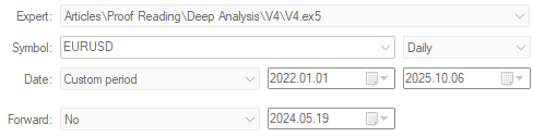
Figure 23: Running the fourth version of our trading application over the same backtest period
Unfortunately, the resulting equity curve shows little to no improvement. The performance appears largely unchanged, and the final account balance has actually declined.
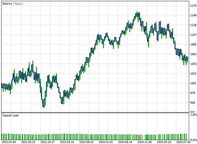
Figure 24: The new features we have added appear to have done very little to give our model a better perspective on the market's state.
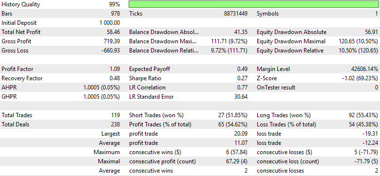
A closer look at the detailed performance statistics reveals that we are now approaching a region of diminishing returns. Both the total net profit and the overall accuracy of the application have dropped. Recall that one of our main objectives was to help the system identify more short opportunities, as the earlier version executed nearly twice as many long positions as short ones. However, this imbalance still persists—the model continues to favor long trades, and the desired improvement in short entries has not yet been realized.
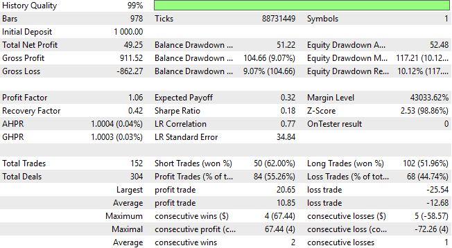
Figure 25: Our detailed results show that our new features may be rendering us diminishing returns
Final Attempt At Improvements
The 22 features we introduced may have been non-linearly related to one another. As a result, the rigid linear model we have relied on so far might not have been flexible enough to capture these complex relationships. To address this, we now define a more powerful non-linear model — specifically, a Random Forest. A Random Forest operates by building an ensemble of multiple decision trees and then averaging their outputs. This allows it to learn non-linear interactions and capture more subtle dependencies within the data that linear models may overlook.
from sklearn.ensemble import RandomForestRegressor
We will now fit our new non-linear model on the same dataset.
model = RandomForestRegressor(random_state=0,max_depth=5,n_estimators=50)
model.fit(data.loc[:,X],data[y])
Finally, export it to an ONNX file.
onnx.save(onnx_proto,"EURUSD 2022-2025 RFR V5.onnx") Implementing The Changes in MQL5
Load the updated ONNX model we have just exported.
//+------------------------------------------------------------------+
//| System resources                                                 |
//+------------------------------------------------------------------+
#resource "\\Files\\EURUSD 2022-2025 RFR V5.onnx" as const uchar onnx_proto[];
Once the model is loaded, we run the application again over the same backtesting window as before.

Figure 26: Evaluating our final version of our trading application over the same test period
Unfortunately, the results show that while profitability did improve slightly compared to the previous version, performance remains significantly below the optimal results achieved with Version 3 of the trading strategy. Furthermore, when we analyze the distribution of short versus long trades, we find that the signal quality has weakened again. The ratio of short to long trades has deteriorated, indicating that the model is once more losing its ability to identify sell opportunities effectively. n other words, we appear to be working harder only to catch up with a simpler model — the one implemented in Version 3 — which achieved stronger and more stable results with less complexity.
Fiugre 27: A detailed analysis of the final version of our trading application reveals that we are retrogressing from our peak performance levels
When we review the equity curve produced by this latest version, we observe no meaningful improvement in stability or profitability. This outcome gives us confidence that we have likely reached a natural stopping point in our exploration of increasingly complex models. Therefore, it may be most prudent to roll back to Version 3 of the application and use it as our stable baseline for future experiments.
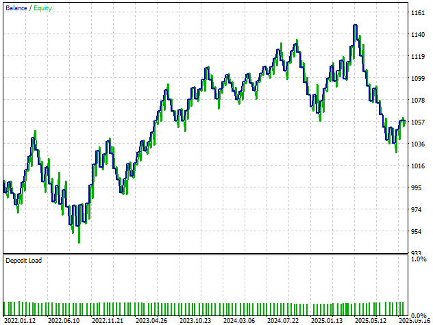
Fiugre 28: The final equity curve we obtained from the final version of our trading application suggests that the third version was optimal
Conclusion
After reading this discussion, the reader gains a deeper understanding of the true challenges that limit the profitability and potential of statistical models in finance. Crucially, success depends less on model complexity and more on methodology—how models are designed, applied, and interpreted.
Pursuing the most advanced models or largest datasets does not guarantee better results; it can even lead to unnecessary costs and diminishing returns. A simple model, applied intelligently, often outperforms a complex one built on flawed assumptions. Model performance is shaped not only by mathematics, but also by the objectives, evaluation framework, and design choices imposed on it. In many cases, methodology itself is the hidden constraint—the “elephant in the room.”
For decades, financial modeling has relied on fixed relationships and rigid forecasting horizons, despite markets being inherently dynamic. When models fail, it is often not because they cannot learn, but because they are tasked with the wrong objective or taught via an unsuitable approach.
This discussion underscores the importance of careful experimentation, diligence, and methodological rigor in applying machine learning to finance. When progress stalls, the solution is not always a bigger model or more data; sometimes the key is simply identifying a better target or refining the process. Thoughtful methodology, rather than sheer complexity, unlocks the true potential of statistical models.
| File Name | File Description |
|---|---|
| Benchmark.mq5 | The benchmark version of our application was not profitable, but established key performance indicators for us to outperform. |
| V1.mq5 | The first version of our application was built according to classical techniques, but failed to produce profitable results in the backtest. |
| V2.mq5 | The second version of our application broke away from classical modelling tecniques and modelled the moving average indicator with marginal success. |
| V3.mq5 | The best version of the application we discovered from our discussion, it modelled the moving average indicator at multiple horizons and traded the implied slope. |
| V4.mq5 | The fourth version of the application kept the same target as the third version but used more data. This change in methodology limited our profitability. |
| V5.mq5 | The final version of our application employed a non-linear learner to model the larger dataset. While it was profitable than the fourth version of our application it failed to match the performance of the third version. |
| Deep_Analysis_V5.ipynb | The jupyter notebook we used to analyze the market data we fetched four our discussion. |
Warning: All rights to these materials are reserved by MetaQuotes Ltd. Copying or reprinting of these materials in whole or in part is prohibited.
This article was written by a user of the site and reflects their personal views. MetaQuotes Ltd is not responsible for the accuracy of the information presented, nor for any consequences resulting from the use of the solutions, strategies or recommendations described.

- Free trading apps
- Over 8,000 signals for copying
- Economic news for exploring financial markets
You agree to website policy and terms of use