Bacterial Evolutionary Algorithm (BEA)
 81
 0

Contents
Introduction
For centuries, populations of living organisms facing limited resources have been solving the same problem: finding, within the space of possible forms, those that ensure survival and preserving them. That is precisely why biology remains a rich source of metaphors for population-based algorithms: natural selection inspired genetic algorithms, swarm behavior inspired swarm intelligence methods, and predator hunting and flock migration inspired dozens of specific approaches explored in this series. Today, we are turning our attention to the organisms that evolve faster than any others on the planet — and according to rules that differ significantly from the parent-offspring pattern we are accustomed to. Let's talk about bacteria.
Bacterial evolution is interesting because it involves a mechanism that is almost entirely absent in higher organisms. This is horizontal gene transfer. Bacteria transfer useful DNA fragments to one another directly, bypassing reproduction: through conjugation, plasmids, and the uptake of free genes from the environment. In a single exchange, a neighboring cell can acquire a ready-made, selection-tested segment of the genome — such as an antibiotic resistance gene — and put it to use immediately. This is the secret behind the phenomenal speed of bacterial adaptation: a beneficial discovery spreads throughout the population not over generations, but almost instantly. From an optimization perspective, this idea is appealing: if a successful part of a solution can be copied directly between individuals, the search can accelerate in situations where a classical genetic algorithm would otherwise have to wait for a series of crossovers.
Here, however, we encounter a terminological distinction that needs to be clarified from the outset: the name “Bacterial Evolutionary Algorithm” is used in the literature for two completely different algorithms that are regularly confused with one another. The first one dates back to Chisato Numaoka’s 1996 paper, “Bacterial Evolution Algorithm for Rapid Adaptation”: strictly speaking, it is not an optimizer for continuous functions, but rather an agent-based model from the field of artificial life. In this model, a colony of adaptive bacteroid agents adapts to a constantly changing environment, with the environment itself performing selection through agent deaths, generally without regard to the agents’ own fitness function. The model is elegant and designed for rapid readaptation to a moving optimum, but its transfer to a static test bench requires such a liberal interpretation that the result is, in essence, a different algorithm. A separate article will be devoted to this branch — the true Numaoka model — because its nature is fundamentally different.
The second algorithm — the one commonly referred to as BEA in the field of optimization — was proposed by Norberto Nawa and Takeshi Furuhashi in 1999. This branch later gave rise to the bacterial memetic algorithm and its discrete variants for the traveling salesman problem. It is this optimization variant of the Nawa–Furuhashi BEA that we will implement in our C_AO framework. Let's test it on the Hilly, Forest, and Megacity test functions, run it through a composite anti-cheat test, and analyze how the algorithm behaves as the problem dimensionality increases. We will leave Numaoka's historical model for later, noting it here only as an alternative branch to revisit.
Implementation of the Algorithm
BEA is based on the observation that, in bacteria, two independent mechanisms are responsible for variability and the exchange of beneficial traits, and both can be framed in terms of optimization. Point mutations in the genome give rise to local variations — this is a tool for fine-tuning an existing solution. Horizontal transfer spreads successful fragments throughout the colony — it is a tool for sharing experience among solutions. Nawa and Furuhashi formalized these two principles as two operators, and understanding the algorithm boils down to understanding what each of them does.
In terms of optimization, each bacterium is an individual in the population, and its chromosome is a coordinate vector in the search space. The chromosome is conceptually divided into segments: contiguous blocks of coordinates, each processed as a single unit. Segmentation is essential because it transforms mutation from a blind, random perturbation into a directed, coordinate-wise (or, more precisely, block-wise) search.
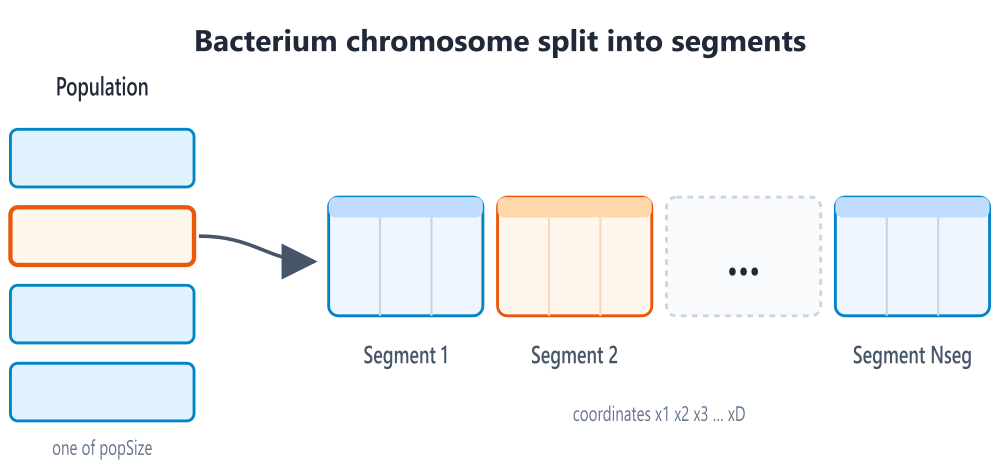
Figure 1. A bacterial chromosome is a coordinate vector in the search space, conceptually divided into segments (contiguous blocks of coordinates)
The figure above shows a bacterium as an individual in a population of size popSize and the segment-based organization of its chromosome.
Bacterial mutation. The first operator is responsible for local optimization within a single chromosome and is applied to each bacterium in the population in turn. A single bacterium is taken, and several copies — clones — are made from it. The chromosome is then processed segment by segment, and the same cycle is performed for each segment. In all but one of the clones, the coordinates of the current segment are randomly regenerated, while one clone remains unchanged — it preserves the segment's current values. After that, all clones are evaluated using the fitness function, and the best one is selected from among them. Its version of this segment is transferred to all other clones, preserving the improvement found in this region of the chromosome. The procedure then moves on to the next segment, and so on until the end of the chromosome. Once all segments have been processed, the original bacterium is replaced by the resulting best clone.
The key detail here is that one clone is left unchanged at each step. Thanks to this, the current incumbent is always included in the set of options being compared, so the best clone is never worse than the original bacterium. This gives bacterial mutation an important property: the bacterium's fitness is monotonically nondecreasing during mutation. The operator functions as a built-in local search — it can only improve an individual or leave it as is, but it cannot worsen it. This is precisely why BEA does not suffer from the problem — common in genetic algorithms — of losing a good solution during mutation: here, mutation is not a probabilistic perturbation, but segment-by-segment optimization that deterministically preserves or improves fitness.
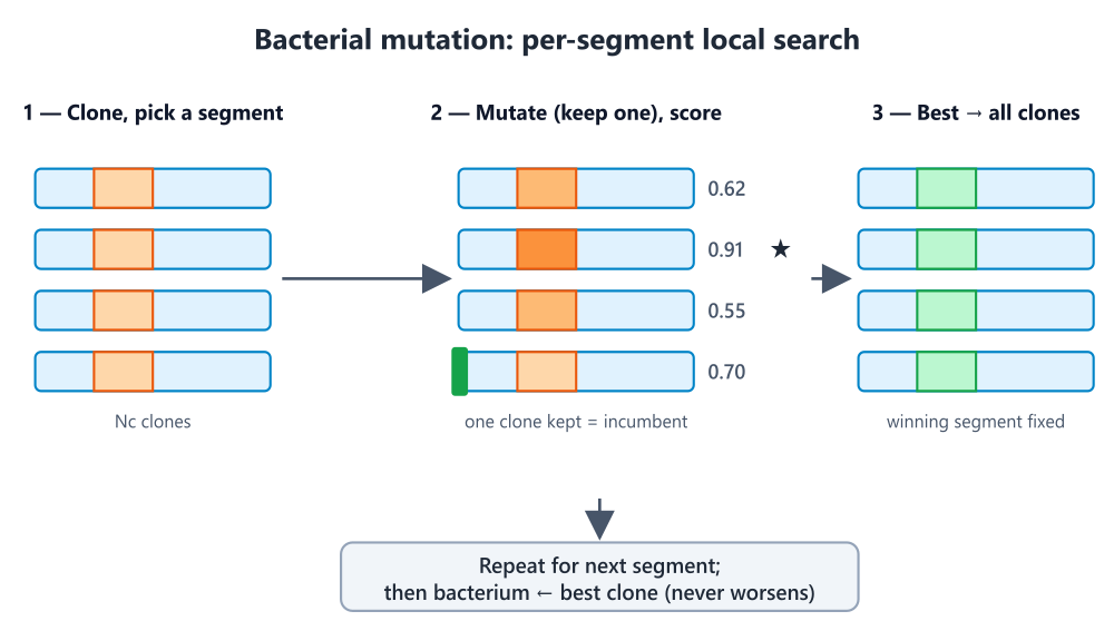
Figure 2. Bacterial mutation as segment-by-segment local optimization.
Let's look at Figure 2. Nc clones are created from the bacterium (1); in the selected segment, the coordinates are randomly regenerated in all clones except one, which remains unchanged and retains the current incumbent; all clones are evaluated (2); the best clone's version of the segment is propagated to all clones (3). Since the incumbent is always included among the candidates being compared, the resulting bacterium is never worse than the original one — fitness is monotonically nondecreasing during mutation. The procedure is repeated for each segment.
Gene transfer. The second operator is responsible for the exchange of information between individuals and simulates the very horizontal gene transfer that makes bacterial evolution so rapid. First, the entire population is sorted by fitness and divided into two halves — the strong half, which includes the best bacteria, and the weak half. The transfer process is then repeated multiple times: a source bacterium is randomly selected from the strong half, a recipient bacterium from the weak half, and a contiguous block of coordinates from the source is copied into the recipient, replacing the corresponding section of its chromosome. The number of such transfer events per generation is specified by a separate parameter.
In essence, gene transfer works differently than crossover in a classical genetic algorithm. Crossover is a form of vertical transmission: traits are passed down from parents to offspring, and a favorable combination spreads only through reproduction, generation after generation. Gene transfer is horizontal: a beneficial fragment is copied directly from a fit individual to an unfit one, here and now, without producing offspring. This allows useful solution blocks to spread rapidly throughout the population and makes lagging individuals more similar in structure to the leaders. If bacterial mutation is intensification — moving each individual further toward a local optimum — then gene transfer is diversification through exchange: a way to prevent weak bacteria from getting stuck in unpromising regions by passing on proven fragments from strong ones.
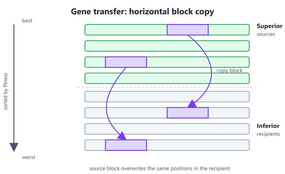
Figure 3. Gene transfer as horizontal exchange.
The population is sorted by fitness and divided into a strong half (sources) and a weak half (recipients). A block of coordinates from a randomly selected source is copied into a randomly selected recipient, replacing the corresponding positions in its chromosome. Unlike vertical inheritance in crossover, a beneficial fragment spreads directly and immediately, making lagging individuals more similar in structure to the leaders.
General outline. The algorithm, composed of two operators, follows a simple loop. The population is initialized randomly and evaluated. Then, until the evaluation budget is exhausted, each generation begins by applying bacterial mutation to all bacteria in turn, completing local optimization of each individual segment by segment. Next, the specified number of gene transfer events is carried out, shuffling the identified blocks between strong and weak bacteria. The globally best solution is stored separately and is not lost during subsequent transformations.
initialize population randomly
evaluate population
while the evaluation budget is not exhausted:

    # --- bacterial mutation (local optimization of each individual) ---
    for each bacterium b:
        create Nc clones of bacterium b
        for each chromosome segment:
            in all clones except one, regenerate the segment randomly
            evaluate all clones
            spread the best segment variant to all clones
        b <- best clone               # incumbent in the set => b does not worsen

    # --- gene transfer (horizontal exchange of blocks) ---
    sort population; divide into strong and weak halves
    repeat Ninf times:
        source  <- random bacterium from the strong half
        recipient  <- random bacterium from the weak half
        copy the coordinate block from the source to the recipient

    update the globally best solution
It is worth noting in advance a particular feature that will be key during implementation. BEA is an algorithm with a heterogeneous and rather computationally expensive generation process: bacterial mutation requires nested evaluations of the fitness function, since each segment of each clone must be evaluated before moving on to the next segment. This does not fit neatly into the "one batch of evaluations per generation" pattern used by our test bench. This will require careful phase-based organization of the computations, as well as accurate accounting of calls to the fitness function — otherwise, comparing BEA with other algorithms under a fixed budget will be invalid. We will discuss exactly how we will solve this problem within the C_AO framework in the next section, which is devoted to implementation.
All algorithms in the series are contained within a single C_AO framework, and its contract is extremely simple. At each epoch, the external loop of the test bench calls the Moving method, which populates the coordinates of all agents in the population — the array a[i].c; the test bench then evaluates each agent using the fitness function, storing the result in a[i].f. Next, the Revision method is called to read these evaluations and update the algorithm's internal state. A key consequence of this contract is that, over the course of a single epoch, the fitness function is called exactly popSize times — once per agent, and no more, no less.
This is where the difficulty mentioned at the end of the previous section lies. By its very nature, bacterial mutation requires nested evaluations: when processing a single bacterium, one must evaluate its clones on the current segment, determine the winner, and only then move on to the next segment. This does not fit the pattern of one batch of popSize evaluations per generation, and there are many such batches per BEA generation. Therefore, the class is implemented as a finite state machine: each epoch of the test bench corresponds to a single evaluation slice, and the state variables keep track of the current segment, clone, or transfer operation. In a single epoch, either the same-index clones of all bacteria are evaluated at once, or all bacteria are evaluated after infection — and the population slot a[i].c holds a meaningful candidate in every epoch.
An individual is represented by a structure containing a coordinate vector and a fitness value, and the algorithm’s internal workings consist of arrays of such structures, without flat buffers that require manual indexing:
//+----------------------------------------------------------------------------+
//|                           Structure                                        |
//+----------------------------------------------------------------------------+
struct S_BEA_Ind
 {
  double c           [];   // coordinates (valid, already processed through SeInDiSp)
  double             f;      // fitness

  void               Init(int coords)
   {
    ArrayResize(c, coords);
    f = -DBL_MAX;
   }
 };
Three arrays are stored at the class level. The first, bact[] of size popSize, holds the committed bacteria — the current population. The second, clone[] of size popSize * Nc, holds the working clones: Nc consecutive slots are allocated to each bacterium, and clone j of bacterium b is stored at index b * Nc + j. The third array, ord[], of size popSize, is an auxiliary array of indices used for sorting during gene transfer. The variables phase, segIdx, cloneIdx, and transIdx define the state of the state machine: the phase (mutation or transfer), the current segment, the current clone slice, and the current transfer epoch.
//+------------------------------------------------------------------+
//|                          Class                                   |
//+------------------------------------------------------------------+
class C_AO_BEA : public C_AO
 {
public:
                    ~C_AO_BEA() {}
                     C_AO_BEA()
   {
    ao_name = "BEA";
    ao_desc = "Bacterial Evolutionary Algorithm";
    ao_link = "https://www.mql5.com/ru/users/joo";

    popSize   = 10;     // number of bacteria
    Nc        = 2;      // new mutants per segment per bacterium (>=1)
    Nseg      = 10;     // number of chromosome segments
    nTrans    = 2;      // gene transfer epochs per generation
    transFrac = 0.2;    // length of the transferred block as a fraction of coords (0..1]

    ArrayResize(params, 5);
    params [0].name = "popSize";
    params [0].val = popSize;
    params [1].name = "Nc";
    params [1].val = Nc;
    params [2].name = "Nseg";
    params [2].val = Nseg;
    params [3].name = "nTrans";
    params [3].val = nTrans;
    params [4].name = "transFrac";
    params [4].val = transFrac;
   }

  void               SetParams()
   {
    popSize   = (int)params [0].val;
    Nc        = (int)params [1].val;
    Nseg      = (int)params [2].val;
    nTrans    = (int)params [3].val;
    transFrac =      params [4].val;

    //--- safeguards
    if(popSize   < 1)
      popSize   = 1;
    if(Nc        < 1)
      Nc        = 1;     // number of new mutants per segment
    if(Nseg      < 1)
      Nseg      = 1;
    if(nTrans    < 0)
      nTrans    = 0;
    if(transFrac <= 0.0)
      transFrac = 0.01;
    if(transFrac >  1.0)
      transFrac = 1.0;
   }

  bool               Init(const double &rangeMinP  [],
                          const double &rangeMaxP  [],
                          const double &rangeStepP [],
                          const int     epochsP = 0);

  void               Moving();
  void               Revision();

  //--- visible parameters
  int                Nc;          // clones
  int                Nseg;        // segments
  int                nTrans;      // gene transfer epochs
  double             transFrac;   // fraction of coords for the transfer block

private:
  //--- phases of the finite-state machine
  enum E_Phase { PH_MUT = 0, PH_TRANS = 1 };
  E_Phase            phase;
  int                segIdx;      // current segment undergoing mutation
  int                cloneIdx;    // current clone (evaluation slice) during mutation
  int                transIdx;    // current transfer epoch

  //--- data (arrays of structures)
  S_BEA_Ind          bact  [];    // [popSize]       — committed bacteria
  S_BEA_Ind          clone [];    // [popSize * Nc]  — working clones
  int                ord   [];    // [popSize]       — sorting indices

  int                transLen;    // transfer block length (from transFrac)

  //--- auxiliary
  void               SegBounds(int s, int &lo, int &hi);
  void               BuildClonesForSeg(int s);
  void               DoGeneTransfer();
 };
After the standard framework initialization, the Init method does three things. It caps the number of segments at the problem dimensionality (Nseg cannot exceed coords) and calculates the absolute length of the transfer block from the fraction transFrac. This is an important detail because the class parameters are fixed across all three tests, while the problem dimensionality varies from test to test; defining the block length as a fraction of the coordinates makes it scalable. Next, arrays of structures are created. The initial population is then initialized by sampling each coordinate uniformly from its allowed range, after which the state machine is reset to the start of the mutation phase.
//+------------------------------------------------------------------+
//|                              Init                                |
//+------------------------------------------------------------------+
bool C_AO_BEA::Init(const double &rangeMinP  [],
                    const double &rangeMaxP  [],
                    const double &rangeStepP [],
                    const int     epochsP = 0)
 {
  if(!StandardInit(rangeMinP, rangeMaxP, rangeStepP))
    return false;

//--- no more segments than coordinates
  if(Nseg > coords)
    Nseg = coords;

//--- transfer block length
  transLen = (int)MathRound(transFrac * coords);
  if(transLen < 1)
    transLen = 1;
  if(transLen > coords)
    transLen = coords;

//--- buffers (arrays of structures)
  ArrayResize(bact,  popSize);
  ArrayResize(clone, popSize * Nc);
  ArrayResize(ord,   popSize);

  for(int i = 0; i < popSize;      i++)
    bact  [i].Init(coords);
  for(int i = 0; i < popSize * Nc; i++)
    clone [i].Init(coords);

//--- initial random population of bacteria
  for(int i = 0; i < popSize; i++)
   {
    for(int c = 0; c < coords; c++)
      bact [i].c [c] = u.SeInDiSp(u.RNDfromCI(rangeMin [c], rangeMax [c]),
                                  rangeMin [c], rangeMax [c], rangeStep [c]);
    bact [i].f = -DBL_MAX;
   }

//--- initial state of the state machine
  phase    = PH_MUT;
  segIdx   = 0;
  cloneIdx = 0;
  transIdx = 0;

  return true;
 }
Chromosome segmentation. The segment boundaries are calculated so that the remaining coordinates are evenly distributed among the segments:
//+------------------------------------------------------------------+
//|   SegBounds — the bounds of segment s in [lo, hi) with uniform   |
//|   distribution of the remaining coordinates across segments      |
//+------------------------------------------------------------------+
void C_AO_BEA::SegBounds(int s, int &lo, int &hi)
 {
  lo = (int)((long)s       * coords / Nseg);
  hi = (int)((long)(s + 1) * coords / Nseg);
  if(lo < 0)
    lo = 0;
  if(hi > coords)
    hi = coords;
 }
It is worth noting the approach taken here: the number of segments, Nseg, is specified as a parameter, and the segment length is derived from it. The alternative — fixing the segment length — would cause the number of segments to explode at high problem dimensionality, driving up the generation cost as well. However, with a fixed number of segments, the mutation cost in fitness function calls does not depend on dimensionality, which, as we will see below, is essential for a fair comparison.
The mutation phase: the first deviation from the canonical formulation. This is where the implementation deliberately diverges from the canonical formulation by Nawa and Furuhashi, and this divergence warrants a detailed explanation. In the canonical formulation, one clone is left unchanged for each segment — it carries the current version of the segment and ensures that the best clone will be no worse than the original bacterium. This unchanged clone serves as a safety net for the incumbent: it is always included among the options being compared.
In our framework, this safety net is costly. Since the test bench uses one fitness function call per population slot regardless, an unchanged clone occupies a slot spent re-evaluating an already known value: the fitness of an untouched copy of a bacterium equals that of the bacterium itself, so recalculating it is pointless. Therefore, the implementation regenerates the segment in all clones and preserves the incumbent differently — by storing its fitness in bact.f and comparing the best clone's fitness against that value at the commit stage. Clone construction therefore does not set aside a reference copy:
//+------------------------------------------------------------------------------+
//|   BuildClonesForSeg — create Nc clones of each bacterium and                 |
//|   randomly regenerate the coordinates of segment s in ALL clones.            |
//|   The incumbent is not stored as a separate clone: its fitness is stored in  |
//|   bact.f and is compared during commit (see Revision).                       |
//+------------------------------------------------------------------------------+
void C_AO_BEA::BuildClonesForSeg(int s)
 {
  int lo, hi;
  SegBounds(s, lo, hi);

  for(int b = 0; b < popSize; b++)
   {
    for(int j = 0; j < Nc; j++)
     {
      int idx = b * Nc + j;

      //--- a copy of the bacterium outside the segment
      for(int c = 0; c < coords; c++)
        clone [idx].c [c] = bact [b].c [c];

      //--- Regeneration of the segment in ALL clones. The incumbent is stored
      //    separately (bact.f) and is compared during the commit phase—
      //    there is no need to re-evaluate it as a clone, saving FF calls.
      for(int c = lo; c < hi; c++)
        clone [idx].c [c] = u.SeInDiSp(u.RNDfromCI(rangeMin [c], rangeMax [c]),
                                       rangeMin [c], rangeMax [c], rangeStep [c]);

      clone [idx].f = -DBL_MAX;
     }
   }
 }
The transfer phase: the second deviation from the canonical formulation. The second difference is smaller and concerns parameterization. In the canonical formulation, transfer consists of Ninf repetitions, in each of which a randomly selected source from the stronger half infects a randomly selected recipient from the weaker half. In the implementation, it was more convenient to tie transfer to the state machine's epochs: during each of the nTrans transfer epochs, the entire weaker half is infected — each bacterium in it receives one block from a randomly selected source in the stronger half. Sorting is performed using an index array, without physically moving the structures:
//+--------------------------------------------------------------------+
//|   DoGeneTransfer — sorts the population and infects the weak       |
//|   half with blocks from the strong half. Modifies bact[] in place. |
//+--------------------------------------------------------------------+
void C_AO_BEA::DoGeneTransfer()
 {
  if(popSize < 2)
    return;

//--- Sorting indices by bacterial fitness (in descending order)
  for(int i = 0; i < popSize; i++)
    ord [i] = i;

  for(int i = 0; i < popSize - 1; i++)
   {
    int bi = i;
    for(int j = i + 1; j < popSize; j++)
      if(bact [ord [j]].f > bact [ord [bi]].f)
        bi = j;
    int t = ord [i];
    ord [i] = ord [bi];
    ord [bi] = t;
   }

  int half = popSize / 2;
  if(half < 1)
    half = 1;

  int span = coords - transLen + 1;
  if(span < 1)
    span = 1;

//--- Each receiver in the "weak" half receives a block from a random
//    source in the "strong" half
  for(int k = half; k < popSize; k++)
   {
    int dst   = ord [k];
    int src   = ord [u.RNDminusOne(half)];
    int start = u.RNDminusOne(span);

    for(int t = 0; t < transLen; t++)
     {
      int c = start + t;
      if(c < coords)
        bact [dst].c [c] = bact [src].c [c];
     }
   }
 }
The acceptance of transferred genotypes is non-greedy, as described in the literature: an infected bacterium is accepted with its new fitness, regardless of whether that fitness has improved or worsened. This is intentional — transfer is meant to mix genetic material, not just improve it, and a temporary decline in an individual bacterium's fitness is acceptable here. The best solution found so far is not compromised: in Revision, it is stored separately in cB / fB immediately after each slot is evaluated, so even an unsuccessful transfer cannot cause the best solution found to be lost — this is ensured by the framework's elitism.
The phase itself is spread across epochs using a state machine. In Moving, at the start of a segment (when cloneIdx is zero), all clones for the current segment are created; then, at each epoch, one clone slice — the same-index clone at cloneIdx from every bacterium — is loaded into the population slots:
//+-------------------------------------------------------------------------+
//|                            Moving                                       |
//|   Fills the slots a[i].c with candidates to be evaluated in this epoch. |
//+-------------------------------------------------------------------------+
void C_AO_BEA::Moving()
 {
//--- First run: bacteria → slots for initial FF evaluation
  if(!revision)
   {
    for(int i = 0; i < popSize; i++)
      for(int c = 0; c < coords; c++)
        a [i].c [c] = u.SeInDiSp(bact [i].c [c], rangeMin [c], rangeMax [c], rangeStep [c]);
    return;
   }

  if(phase == PH_MUT)
   {
    //--- At the start of the segment, we create clones
    if(cloneIdx == 0)
      BuildClonesForSeg(segIdx);

    //--- Load the current clone of each bacterium into the slots
    for(int b = 0; b < popSize; b++)
     {
      int idx = b * Nc + cloneIdx;
      for(int c = 0; c < coords; c++)
        a [b].c [c] = clone [idx].c [c];
     }
   }
  else // PH_TRANS
   {
    //--- Infect the weaker half and load the bacteria into the slots
    DoGeneTransfer();

    for(int b = 0; b < popSize; b++)
      for(int c = 0; c < coords; c++)
        a [b].c [c] = bact [b].c [c];
   }
 }
Accurate accounting of fitness function calls. Now it is clear why organizing execution into phases is so important for a fair comparison. The generation cost of BEA, measured in fitness function calls, consists of two components: mutation requires Nseg * Nc * popSize evaluations (each of the Nseg segments tests Nc clones for each of the popSize bacteria), and transfer requires nTrans * popSize. Crucially, neither of these depends on the problem dimensionality: whether coords is ten or a thousand, the generation cost remains the same. As a result, BEA uses its total budget of 10,000 evaluations according to the same rules as the other algorithms in the series, and the comparison under a fixed budget remains fair — no algorithm gains a hidden advantage because its “generation” actually contains a different number of evaluations.
In Revision, the evaluations for this slice are written to the corresponding clones, the cloneIdx counter is incremented, and once all Nc clones for the segment have been evaluated, the best one is selected for each bacterium and committed according to the rule described above. After that, the state machine moves on to the next segment, and once it has gone through all the segments, it proceeds to the gene transfer phase.
The best clone is committed only if it has actually outperformed the bacterium:
//+------------------------------------------------------------------+
//|                           Revision                               |
//|   Reads a[i].f, updates cB/fB, and advances the state machine.   |
//+------------------------------------------------------------------+
void C_AO_BEA::Revision()
 {
//--- global best (elitism: the best is not lost during transfer)
  for(int i = 0; i < popSize; i++)
   {
    if(a [i].f > fB)
     {
      fB = a [i].f;
      ArrayCopy(cB, a [i].c, 0, 0, coords);
     }
   }

//--- Initial fitness recording of bacteria
  if(!revision)
   {
    for(int i = 0; i < popSize; i++)
      bact [i].f = a [i].f;

    revision = true;
    phase    = PH_MUT;
    segIdx   = 0;
    cloneIdx = 0;
    transIdx = 0;
    return;
   }

  if(phase == PH_MUT)
   {
    //--- Save the fitness of the evaluated slice of clones
    for(int b = 0; b < popSize; b++)
      clone [b * Nc + cloneIdx].f = a [b].f;

    cloneIdx++;

    //--- Segment fully evaluated -> Commit the best clone
    if(cloneIdx >= Nc)
     {
      for(int b = 0; b < popSize; b++)
       {
        int    best = 0;
        double bf   = clone [b * Nc + 0].f;
        for(int j = 1; j < Nc; j++)
         {
          double cf = clone [b * Nc + j].f;
          if(cf > bf)
           {
            bf = cf;
            best = j;
           }
         }

        //--- Commit the best mutant ONLY if it has outperformed
        //    the incumbent; otherwise, the bacterium remains the same (monotonicity
        //    of mutation is preserved without re-evaluating the incumbent as a clone)
        if(bf > bact [b].f)
         {
          int bi = b * Nc + best;
          for(int c = 0; c < coords; c++)
            bact [b].c [c] = clone [bi].c [c];
          bact [b].f = bf;
         }
       }

      cloneIdx = 0;
      segIdx++;

      //--- All segments have been completed -> gene transfer (or a new generation)
      if(segIdx >= Nseg)
       {
        segIdx = 0;
        if(nTrans > 0)
         {
          phase = PH_TRANS;
          transIdx = 0;
         }
        else
          phase = PH_MUT;
       }
     }
   }
  else // PH_TRANS
   {
    //--- We accept infected genotypes (non-greedy)
    for(int b = 0; b < popSize; b++)
      bact [b].f = a [b].f;

    transIdx++;
    if(transIdx >= nTrans)
     {
      phase    = PH_MUT;
      segIdx   = 0;
      cloneIdx = 0;
     }
   }
 }
It is important to understand that this is not a cosmetic tweak, but a substantive improvement. When Nc = 2, the canonical scheme produces one unaltered clone and one mutant per segment; that is, it tests only one new variant. Our scheme produces two mutants at the same cost — two function calls. The slot freed up by avoiding re-evaluation of the incumbent is filled by an additional fresh candidate, and this is precisely what raised the baseline configuration's final score in our runs from approximately 50 to 53 percent. At the same time, the monotonicity of mutation is fully preserved: the condition if (bf > bact.f) means that the bacterium either improves or remains unchanged, but never deteriorates — precisely the property for which an unchanged clone was retained in the canonical algorithm.
Parameters. The class has five visible parameters. The population size, popSize, is the number of bacteria. The number of clones, Nc, is the number of new mutants tested on each segment. The number of segments, Nseg, determines the granularity of blockwise mutation. The number of transfer epochs, nTrans, specifies the intensity of horizontal exchange per generation. Finally, the fraction transFrac determines the length of the transferred block relative to the problem dimensionality. We will examine their relationship to the budget — specifically, the trade-off between the quality of a single generation and the number of generations that can fit within a fixed budget — when we analyze the test results.
Test Results
Across all of our test functions, the algorithm achieved a score of 53.13% with a population size of 10 individuals.BEA|Bacterial Evolutionary Algorithm|10.0|2.0|10.0|2.0|0.2|
=============================
5 Hilly's; Func runs: 10000; result: 0.9217077440618244
25 Hilly's; Func runs: 10000; result: 0.5961506596554828
500 Hilly's; Func runs: 10000; result: 0.2934090356286264
=============================
5 Forest's; Func runs: 10000; result: 0.9690648482875481
25 Forest's; Func runs: 10000; result: 0.44500075828106833
500 Forest's; Func runs: 10000; result: 0.08233566231751262
=============================
5 Megacity's; Func runs: 10000; result: 0.9053333333333334
25 Megacity's; Func runs: 10000; result: 0.4317333333333332
500 Megacity's; Func runs: 10000; result: 0.13676000000000088
=============================
All score: 4.78150 (53.13%)
The anti-cheat test indicates that the reported results genuinely reflect the algorithm's search capability.
BEA|Bacterial Evolutionary Algorithm|10.0|2.0|10.0|2.0|0.2|
=============================
Composite anti-cheat test: Hilly + Forest + Megacity + Peaks + Skin
Coordinates: 10; Epochs: 1000; Repeats: 10
=============================
Run 1/10: 0.9468505530003426
Run 2/10: 0.9621805930887799
Run 3/10: 0.8517460551795464
Run 4/10: 0.968005214717207
Run 5/10: 0.8697467385084419
Run 6/10: 0.9729983388567323
Run 7/10: 0.9703386568386824
Run 8/10: 0.9663920708043637
Run 9/10: 0.9545824368636746
Run 10/10: 0.8336853637354364
=============================
Average result: 0.9296526022 (92.97%)
=============================
Visualization of the BEA algorithm's operation on test functions, as well as on freely chosen functions.

BEA on the Hilly test function

BEA on the Forest test function

BEA on the Megacity test function

BEA on the Peaks test function

BEA on the Ackley test function
Based on the test results, the algorithm ranks 37th in the overall ranking of the best population-based optimization methods.
| cc | AO | Description | Hilly | Hilly Final | Forest | Forest Final | Megacity (discrete) | Megacity Final | Final Result | % of MAX | ||||||
| 10 p (5 F) | 50 p (25 F) | 1,000 p (500 F) | 10 p (5 F) | 50 p (25 F) | 1,000 p (500 F) | 10 p (5 F) | 50 p (25 F) | 1,000 p (500 F) | ||||||||
| 1 | ANS | across neighbourhood search | 1.00000 | 0.88228 | 0.40138 | 2.28366 | 1.00000 | 0.95281 | 0.28092 | 2.23373 | 0.94667 | 0.85733 | 0.22389 | 2.02789 | 6.545 | 72.72 |
| 2 | AMOm | animal migration optimization M | 0.91624 | 0.83603 | 0.46790 | 2.22017 | 0.98482 | 0.92010 | 0.36391 | 2.26883 | 0.91733 | 0.81707 | 0.25177 | 1.98617 | 6.475 | 71.94 |
| 3 | CLA | code lock algorithm (joo) | 0.95139 | 0.86199 | 0.37879 | 2.19217 | 0.99349 | 0.93500 | 0.26497 | 2.19346 | 0.93600 | 0.84267 | 0.24060 | 2.01927 | 6.405 | 71.17 |
| 4 | (P+O)ES | (P+O) evolution strategies | 0.86571 | 0.89539 | 0.39740 | 2.15850 | 0.97761 | 0.89820 | 0.26878 | 2.14459 | 0.92133 | 0.80240 | 0.23952 | 1.96325 | 6.266 | 69.62 |
| 5 | SDSm | stochastic diffusion search M | 0.95195 | 0.84944 | 0.36249 | 2.16388 | 0.98061 | 0.88457 | 0.22112 | 2.08630 | 0.92267 | 0.79013 | 0.21380 | 1.92660 | 6.177 | 68.63 |
| 6 | AAm | archery algorithm M | 0.84685 | 0.73320 | 0.42590 | 2.00595 | 0.96709 | 0.77837 | 0.27789 | 2.02335 | 0.86133 | 0.77707 | 0.28712 | 1.92552 | 5.955 | 66.17 |
| 7 | SIA | simulated isotropic annealing (joo) | 0.93543 | 0.86504 | 0.38483 | 2.18530 | 0.94069 | 0.80609 | 0.23835 | 1.98513 | 0.86400 | 0.66160 | 0.19536 | 1.72096 | 5.891 | 65.46 |
| 8 | TETA | time evolution travel algorithm (joo) | 0.91452 | 0.86369 | 0.25579 | 2.03400 | 0.99654 | 0.91291 | 0.14394 | 2.05339 | 0.85467 | 0.82213 | 0.10443 | 1.78123 | 5.869 | 65.21 |
| 9 | ESG | evolution of social groups (joo) | 0.98111 | 0.79857 | 0.31167 | 2.09135 | 0.98954 | 0.82270 | 0.15032 | 1.96256 | 0.92133 | 0.73440 | 0.15315 | 1.80888 | 5.863 | 65.14 |
| 10 | CTA | comet tail algorithm (joo) | 0.92435 | 0.86786 | 0.27838 | 2.07059 | 0.99039 | 0.84571 | 0.19448 | 2.03058 | 0.95467 | 0.69680 | 0.11008 | 1.76155 | 5.863 | 65.14 |
| 11 | COA | coyote_optimization_algorithm | 0.88909 | 0.70681 | 0.32718 | 1.92308 | 0.99467 | 0.85358 | 0.15152 | 1.99977 | 0.88533 | 0.71040 | 0.18981 | 1.78554 | 5.708 | 63.43 |
| 12 | ECBO | enhanced colliding bodies optimization | 0.94024 | 0.72363 | 0.32356 | 1.98743 | 0.99477 | 0.80291 | 0.13056 | 1.92824 | 0.87600 | 0.70160 | 0.17433 | 1.75193 | 5.668 | 62.98 |
| 13 | DA | dialectical algorithm | 0.93117 | 0.75400 | 0.26205 | 1.94722 | 0.98925 | 0.81375 | 0.08662 | 1.88962 | 0.92667 | 0.68107 | 0.11315 | 1.72089 | 5.558 | 61.76 |
| 14 | BBO | biogeography-based optimization | 0.95876 | 0.70609 | 0.35752 | 2.02237 | 0.92981 | 0.70660 | 0.16970 | 1.80611 | 0.87467 | 0.63013 | 0.20813 | 1.71293 | 5.541 | 61.57 |
| 15 | BHAm | black hole algorithm M | 0.79558 | 0.76207 | 0.34682 | 1.90447 | 0.99836 | 0.75798 | 0.13826 | 1.89460 | 0.85067 | 0.64427 | 0.17020 | 1.66514 | 5.464 | 60.71 |
| 16 | HS | harmony search | 0.91420 | 0.69049 | 0.29924 | 1.90393 | 0.97627 | 0.73373 | 0.14193 | 1.85193 | 0.91733 | 0.62720 | 0.15364 | 1.69817 | 5.454 | 60.60 |
| 17 | RFO | royal flush optimization (joo) | 0.80989 | 0.74481 | 0.34546 | 1.90016 | 0.95251 | 0.77926 | 0.15185 | 1.88362 | 0.80400 | 0.66427 | 0.19071 | 1.65898 | 5.443 | 60.48 |
| 18 | BOAm | billiards optimization algorithm M | 0.76177 | 0.72421 | 0.25275 | 1.73873 | 0.90890 | 0.81960 | 0.28853 | 2.01703 | 0.83733 | 0.74613 | 0.09763 | 1.68109 | 5.437 | 60.41 |
| 19 | ASO | anarchy society optimization | 0.73070 | 0.73713 | 0.31195 | 1.77978 | 0.99732 | 0.87700 | 0.17619 | 2.05051 | 0.72000 | 0.68773 | 0.18988 | 1.59761 | 5.428 | 60.31 |
| 20 | EOm | Extremal Optimization_M | 0.76527 | 0.75205 | 0.31908 | 1.83640 | 0.99999 | 0.76426 | 0.12437 | 1.88862 | 0.84133 | 0.64133 | 0.15247 | 1.63513 | 5.360 | 59.56 |
| 21 | ACS | artificial cooperative search | 0.75545 | 0.77162 | 0.31653 | 1.84360 | 1.00000 | 0.80488 | 0.10705 | 1.91193 | 0.76933 | 0.60800 | 0.14157 | 1.51890 | 5.274 | 58.60 |
| 22 | SSG | saplings sowing and growing | 0.75436 | 0.63206 | 0.35935 | 1.74577 | 0.91907 | 0.69694 | 0.19755 | 1.81356 | 0.81867 | 0.60533 | 0.21347 | 1.63747 | 5.197 | 57.74 |
| 23 | AOSm | atomic orbital search M | 0.76184 | 0.68435 | 0.31344 | 1.75963 | 0.90015 | 0.80044 | 0.11501 | 1.81560 | 0.82800 | 0.63280 | 0.15696 | 1.61776 | 5.193 | 57.70 |
| 24 | TSEA | turtle shell evolution algorithm (joo) | 0.95809 | 0.64852 | 0.29571 | 1.90232 | 0.99522 | 0.58104 | 0.10542 | 1.68168 | 0.92133 | 0.52160 | 0.14567 | 1.58860 | 5.173 | 57.48 |
| 25 | DE | differential evolution | 0.96398 | 0.62346 | 0.26089 | 1.84833 | 0.98482 | 0.77018 | 0.11459 | 1.86959 | 0.93067 | 0.36213 | 0.11000 | 1.40280 | 5.121 | 56.90 |
| 26 | BIO | blood inheritance optimization (joo) | 0.72580 | 0.66522 | 0.31228 | 1.70330 | 0.99995 | 0.68125 | 0.11540 | 1.79660 | 0.85467 | 0.59333 | 0.15364 | 1.60164 | 5.102 | 56.69 |
| 27 | (PO)ES | (PO) evolution strategies | 0.73972 | 0.58190 | 0.38896 | 1.71058 | 0.91199 | 0.59975 | 0.21262 | 1.72436 | 0.82400 | 0.56240 | 0.23432 | 1.62072 | 5.056 | 56.18 |
| 28 | BO | bonobo optimizer | 0.75555 | 0.64366 | 0.32657 | 1.72578 | 0.94332 | 0.70442 | 0.13999 | 1.78773 | 0.73467 | 0.61440 | 0.16728 | 1.51635 | 5.030 | 55.89 |
| 29 | SRA | successful restaurateur algorithm (joo) | 0.89010 | 0.63359 | 0.29115 | 1.81484 | 0.96634 | 0.55285 | 0.08914 | 1.60833 | 0.89333 | 0.52800 | 0.13911 | 1.56044 | 4.984 | 55.38 |
| 30 | CRO | chemical reaction optimisation | 0.91281 | 0.65681 | 0.29866 | 1.86828 | 0.90513 | 0.56020 | 0.10939 | 1.57472 | 0.82800 | 0.50133 | 0.14149 | 1.47082 | 4.914 | 54.60 |
| 31 | BCOm | bacterial chemotaxis optimization M | 0.82589 | 0.61733 | 0.31584 | 1.75906 | 0.95296 | 0.63718 | 0.11984 | 1.70998 | 0.76533 | 0.51653 | 0.15800 | 1.43986 | 4.909 | 54.54 |
| 32 | DOA | dream optimization algorithm | 0.78522 | 0.78121 | 0.36036 | 1.92679 | 0.61584 | 0.42117 | 0.12254 | 1.15955 | 0.86667 | 0.72587 | 0.21127 | 1.80381 | 4.890 | 54.33 |
| 33 | ABO | african buffalo optimization | 0.92295 | 0.62528 | 0.29885 | 1.84708 | 0.92992 | 0.57468 | 0.09372 | 1.59832 | 0.73333 | 0.51333 | 0.14324 | 1.38990 | 4.835 | 53.72 |
| 34 | BSA | bird swarm algorithm | 0.94432 | 0.67941 | 0.26401 | 1.88774 | 0.91649 | 0.65619 | 0.12054 | 1.69322 | 0.80933 | 0.33547 | 0.10652 | 1.25132 | 4.832 | 53.69 |
| 35 | TSm | tabu search M | 0.87806 | 0.61040 | 0.28993 | 1.77839 | 0.98116 | 0.52165 | 0.08544 | 1.58825 | 0.82667 | 0.49547 | 0.13552 | 1.45766 | 4.824 | 53.60 |
| 36 | BSA | backtracking search algorithm | 0.87128 | 0.53190 | 0.28675 | 1.68993 | 0.92408 | 0.51602 | 0.09153 | 1.53163 | 0.96000 | 0.47253 | 0.13760 | 1.57013 | 4.792 | 53.24 |
| 37 | BEA | bacterial_evolutionary_algorithm | 0.92170 | 0.59615 | 0.29340 | 1.81125 | 0.96906 | 0.44500 | 0.08233 | 1.49639 | 0.90533 | 0.43173 | 0.13676 | 1.47382 | 4.781 | 53.13 |
| 38 | BWOm | beluga_whale_optimization_M | 0.78488 | 0.56872 | 0.29557 | 1.64917 | 0.91370 | 0.61760 | 0.12988 | 1.66118 | 0.81333 | 0.49946 | 0.15004 | 1.46283 | 4.773 | 53.04 |
| 39 | WOAm | whale optimization algorithm M | 0.93893 | 0.59477 | 0.26695 | 1.80065 | 0.98036 | 0.53873 | 0.07112 | 1.59021 | 0.78667 | 0.47600 | 0.11892 | 1.38159 | 4.772 | 53.02 |
| 40 | ACA | andean_condor_algorithm | 0.78444 | 0.53260 | 0.33108 | 1.64812 | 0.79071 | 0.44960 | 0.10685 | 1.34716 | 0.92266 | 0.67733 | 0.17613 | 1.77612 | 4.771 | 53.02 |
| 41 | CSO | competitive swarm optimizer | 0.85151 | 0.60786 | 0.29896 | 1.75833 | 0.84085 | 0.58491 | 0.11974 | 1.54550 | 0.80000 | 0.48560 | 0.14184 | 1.42744 | 4.731 | 52.57 |
| 42 | FBA | fractal-based algorithm | 0.69419 | 0.64267 | 0.28955 | 1.62641 | 0.99812 | 0.54905 | 0.08705 | 1.63422 | 0.76133 | 0.51253 | 0.13689 | 1.41075 | 4.671 | 51.90 |
| 43 | ECOi | eco-inspired evolutionary algorithm | 0.78817 | 0.54402 | 0.29360 | 1.62579 | 0.88996 | 0.46592 | 0.09747 | 1.45335 | 0.78533 | 0.45173 | 0.14295 | 1.38001 | 4.459 | 49.54 |
| 44 | BSO | brain storm optimization | 0.92207 | 0.57625 | 0.29732 | 1.79564 | 0.80764 | 0.42508 | 0.09448 | 1.32720 | 0.77200 | 0.36533 | 0.13065 | 1.26798 | 4.391 | 48.79 |
| 45 | CAm | camel algorithm M | 0.71534 | 0.56917 | 0.35985 | 1.64436 | 0.84094 | 0.47174 | 0.10850 | 1.42118 | 0.70400 | 0.41947 | 0.19563 | 1.31910 | 4.385 | 48.72 |
| RW | random walk | 0.49970 | 0.32333 | 0.25791 | 1.08094 | 0.30754 | 0.11470 | 0.04400 | 0.46624 | 0.36133 | 0.17013 | 0.10244 | 0.63390 | 2.181 | 24.23 | |
Conclusions
The Nawa–Furuhashi version of the bacterial evolutionary algorithm proved to be clear and straightforward, with no hidden geometric tricks and predictable behavior whose underlying causes are easy to understand. Overall, across the three test functions, it achieved a score of 53.13% with a small population. This figure should be read not as a single number, but as the combined outcome of two very different stories at different dimensionalities.
BEA performs well in low-dimensional spaces. With ten coordinates, it achieves results in the top third of the table — around 0.92 on Hilly, 0.97 on Forest, and 0.91 on Megacity. The explanation lies in the very nature of bacterial mutation: when a segment consists of one or two coordinates, segment-by-segment regeneration becomes an almost coordinate-wise global search, which works extremely well on multimodal functions by sampling coordinate values across the entire range and retaining the best. Gene transfer adds to this the rapid exchange of successful blocks, and together they result in strong convergence.
As dimensionality increases, the results naturally deteriorate, and here we encounter a structural limitation rather than inadequate tuning. Since the number of segments is fixed, with 1,000 coordinates each segment spans about a hundred dimensions, and randomly regenerating such a block all at once almost never produces a solution better than the incumbent. Mutation effectively stalls, leaving gene transfer to do all the work; yet gene transfer, in turn, has nothing to recombine in a nearly random population. Crucially, this is not a matter of budget: even with an unlimited number of evaluations, coarse block regeneration in high dimensions does not improve the solution. This is an inherent property of the algorithm, not an implementation flaw, and that is exactly how it is presented in the article.
A composite anti-cheat test consisting of five dissimilar functions confirmed that the algorithm does not take shortcuts: its result on the composite does not exceed its results on individual functions of the same dimensionality. In other words, BEA does not exploit the axial symmetry of the test bench and genuinely optimizes each coordinate pair. This follows from both mutation and transfer operating strictly block by block, without any hidden multiplication of the entire vector by a common scalar.
If one were to describe BEA in a single sentence, it would be a carefully designed local optimizer with a mechanism for rapidly sharing discoveries, very well suited to problems of moderate dimensionality but structurally limited at high dimensionalities. Its central idea — the horizontal transfer of solution blocks directly between individuals — remains valuable and transferable: it demonstrates how to accelerate the spread of successful fragments without waiting for a series of crossovers.
And here it is worth returning to the fork in the road where we began. The Nawa–Furuhashi optimization branch discussed in this article is just one of two branches known as bacterial algorithms. The other branch, Chisato Numaoka's original 1996 model, works in a fundamentally different way: it is not an optimizer of static functions, but an agent-based model of rapid adaptation in which the environment carries out selection through agent deaths, while the colony itself is designed to survive in constantly changing conditions. Testing such a model on a static test bench means asking it to do something it was not designed for. Therefore, a separate article will be devoted to Numaoka's model. We will set up a test bench with a moving optimum and see whether the energy-based mechanism of bacterial adaptation proves its worth there — the very feature that seems redundant on static functions but may prove decisive on non-stationary ones.
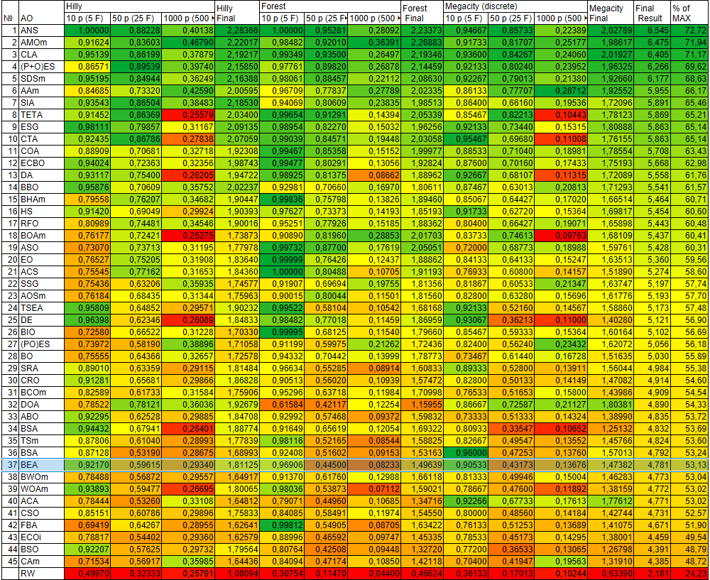
Figure 4. Color-coded ranking of algorithms based on the corresponding tests
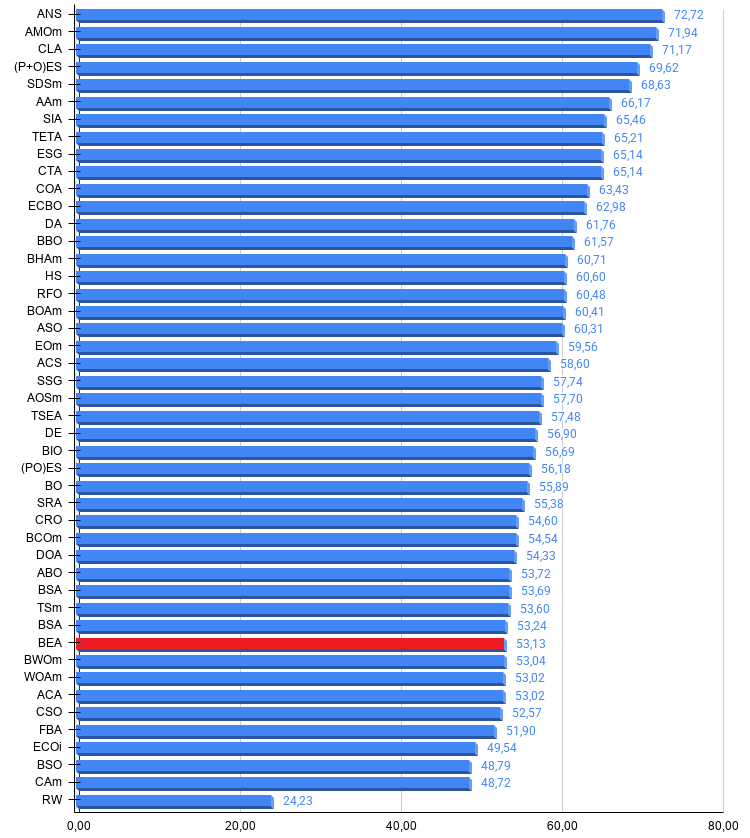
Figure 5. A histogram of the algorithm test results (on a scale from 0 to 100: the higher the score, the better, where 100 is the maximum possible theoretical result); the archive contains a script for calculating the ranking table
Pros and cons of the BEA algorithm:
Pros:
- Good search capabilities.
- Consistency of results (low variability).
Cons:
- A large number of external parameters.
An archive containing the latest versions of the algorithm source code is attached to the article. The author of this article is not responsible for the absolute accuracy of the descriptions of canonical algorithms; many of them have been modified to improve search capabilities. The conclusions and judgments presented in the articles are based on the results of the experiments conducted.
Programs used in this article
| # | Name | Type | Description |
|---|---|---|---|
| 1 | #C_AO.mqh | Include file | Parent class of population-based optimization algorithms |
| 2 | #C_AO_enum.mqh | Include file | Enumeration of population-based optimization algorithms |
| 3 | TestFunctions.mqh | Include file | Test function library |
| 4 | TestStandFunctions.mqh | Include file | Test bench function library |
| 5 | TestStand3D.mqh | Include file | 3D visualization panel for a test bench |
| 6 | Utilities.mqh | Include file | Utility function library |
| 7 | CalculationTestResults.mqh | Include file | Script for calculating results for the comparison table |
| 8 | Test_AO_All.mq5 | Script | Unified test bench for all population-based optimization algorithms |
| 9 | Test_AO_AntiCheat | Script | Anti-cheat test for optimization algorithms |
| 10 | Simple use of population optimization algorithms.mq5 | Script | Simple example of using population-based optimization algorithms without visualization |
| 11 | Test_AO_BEA.mq5 | Script | Test bench for BEA |
Translated from Russian by MetaQuotes Ltd.
Original article: https://www.mql5.com/ru/articles/23232
Warning: All rights to these materials are reserved by MetaQuotes Ltd. Copying or reprinting of these materials in whole or in part is prohibited.
This article was written by a user of the site and reflects their personal views. MetaQuotes Ltd is not responsible for the accuracy of the information presented, nor for any consequences resulting from the use of the solutions, strategies or recommendations described.