Meta-Labeling the Classics (Part 4): Filtering and Sizing MACD Trades

Table of Contents

1. Introduction
2. Quantifying the Failure Mode
3. A Two-Layer Meta-Labeling Framework
4. Contextual Features for the Secondary Classifier
5. Validation Protocol
6. Results
7. Discussion and Limitations
8. Conclusion
9. Attached Files

Introduction

MACD signal-line crossovers fire whenever the difference between a fast and a slow EMA crosses its own smoothed average. The rule does not distinguish a crossover produced by a genuine change in trend velocity from a crossover produced by two converged EMAs oscillating around each other in a range. Both look identical at the moment the lines cross; only the bars that follow reveal which one occurred, and by then the trade is already open.

This is Part 4 of the Meta-Labeling the Classics series. Part 1 applied the meta-labeling framework to RSI, a mean-reversion tool that breaks in trending conditions. Part 2 applied it to the ADX/DI directional movement system, a trend-following tool that breaks in ranging conditions — the structural inverse of Part 1's failure. Part 3 returned to the mean-reversion side with Bollinger Bands, where a bandwidth feature gave the secondary model a direct read on the trending regimes that break the primary signal. MACD is trend-following like ADX/DI, so its failure mode is closer to Part 2 than to Parts 1 or 3. However, the mechanism differs: ADX/DI fails when directional movement lacks persistence, while MACD can trigger on any sign change in the EMA difference, even if it is small and quickly reversed.

The pipeline draws on methods from two series: MetaTrader 5 Machine Learning Blueprint and Feature Engineering for ML. Triple-barrier labeling is covered in Blueprint Part 2, sample-uniqueness weighting in Blueprint Part 5, Bayesian HPO in Blueprint Parts 8–9 (with Part 9), bet sizing in Blueprint Part 10, and session-timing features in Feature Engineering Part 3.

Section 2 quantifies the failure mode on real EURUSD H1 data. Sections 3 through 5 build the two-layer filter, the feature set, and the validation protocol. Sections 6 and 7 report results and state plainly what they do and do not demonstrate.

Quantifying the Failure Mode

Gerald Appel's original MACD uses three EMA spans — 12, 26, and 9 periods — chosen against weekly stock charts in the 1970s. Nothing in the construction adapts those spans, or the signal-line crossover rule itself, to a specific instrument or a specific bar frequency. Applied unmodified to EURUSD H1 data, the rule generates a trade on every sign change of MACD − Signal, with no requirement that the change be large, sustained, or aligned with any broader context.

The panel below shows a real segment from the dataset used in this article: 43,103 hourly EURUSD bars from January 2018 through December 2024. The data comes from a broker export with bid, ask, and mid OHLC, plus spread and tick volume. Mid prices are used for signals, features, and labeling; Section 6 provides the full description. From August 20 to August 23, 2019, price chops inside a roughly 90-pip band before breaking sharply higher in the final hours shown. The MACD and signal lines cross seventeen times in this window — nine long, eight short — each crossover triggering a trade in the opposite direction from the one before it.

from afml.strategies.trading_strategies import MACDStrategy

strat = MACDStrategy()  # fast=12, slow=26, signal=9 (Appel's defaults)
macd_df = strat.compute_macd(df)      # columns: macd, macd_signal, macd_hist
raw_signals = strat.generate_signals(df)  # 1 / -1 / 0, signal-line crossovers only

MACD signal-line crossovers during a ranging stretch

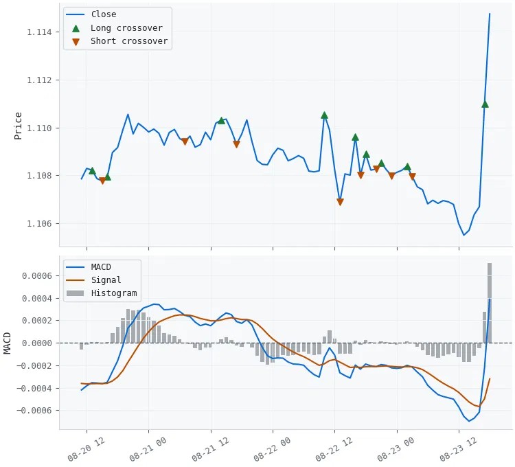
Figure 1. Two-panel illustration of whipsaw crossovers in a ranging stretch

• Panel (a): close price chopping inside a narrow band, with each signal-line crossover marked — green triangles for long, orange for short.
• Panel (b): the MACD line, signal line, and histogram for the same window. Every crossover corresponds to a histogram sign change of a few hundredths of a pip, well inside the noise band of an EMA difference computed on H1 closes.

Over the full out-of-sample test window used in Section 6 (August 2023 through December 2024), the naive rule fires 673 times. Section 6 reports what that costs in drawdown terms. The point here is structural, not statistical: the signal-line crossover event itself carries no explicit information about the magnitude or persistence of the momentum change that produced it — the accompanying MACD and histogram values contain partial information, but the crossover alone does not — so a market that spends any material fraction of its time ranging will feed the rule a steady diet of low-conviction trades indistinguishable, at entry, from the trades that catch a real move.

A Two-Layer Meta-Labeling Framework

The meta-labeling framework from Chapter 3 of Marcos López de Prado's Advances in Financial Machine Learning separates the side decision from the size decision. The primary model — here, the MACD signal-line crossover — continues to generate directional signals exactly as before. A secondary classifier receives each signal along with contextual measurements taken at the signal bar and outputs the probability that the signal will reach its profit-taking barrier before its stop-loss barrier. In this pipeline the classifier's output is used for position sizing via bet_size_probability; signals are not skipped below a confidence threshold — every gated signal is sized, not filtered.

Part 2 of this series added a first layer ahead of the classifier: an Optuna-optimized regime gate that replaced Wilder's fixed ADXR ≥ 25 threshold with a data-driven one, tuned to maximize signal precision on a held-out window. This article carries that same two-layer structure forward, with one difference worth stating plainly rather than leaving implicit.

Wilder specified ADXR ≥ 25 as part of the Directional Movement System itself — Part 2's gate operationalized an author-stated safeguard. Appel specified no equivalent regime filter for MACD. The three gate parameters introduced below are therefore an engineering addition layered onto the classic rule, not the recovery of a threshold the original author intended traders to apply.

That distinction changes the claim this article can honestly make: not "MACD becomes reliable once you apply Appel's own filter," but "MACD's crossover rule accepts a regime filter this cleanly, and here is what imposing one costs and buys."

The gate has three parameters, chosen to mirror Part 2's structure (a magnitude floor, a persistence requirement, and a directional-agreement flag) while fitting MACD's own internal state rather than ADX's:

• min_hist_atr — the MACD histogram must exceed this fraction of ATR(14) at the crossover bar. Mirrors Part 2's minimum DI separation: a floor on how large the momentum change has to be before it counts.
• confirm_bars — the histogram's sign must have held for this many consecutive bars up to and including the crossover bar. Mirrors Part 2's DI lookback: a floor on how long the new regime has to have been in place. Note on timing: because the raw signal fires on the first bar of the new histogram sign, requiring confirm_bars > 1 deliberately delays the gated entry until the new sign has persisted for the required number of bars. This is a confirmation lag, not an instantaneous crossover filter; the trade-off is later entry in exchange for fewer whipsaws.
• zero_line_required — if true, the MACD line's own sign must agree with the trade direction (long only when MACD > 0). A binary regime-agreement flag with no direct ADX analogue.

Optuna's TPE sampler searches this three-parameter space — min_hist_atr over [0.0, 0.6], confirm_bars over {1, 2, 3}, zero_line_required over {True, False}, for 40 trials — to maximize gated-signal precision (the fraction of gated signals whose triple-barrier label is 1) on the first 20% of the history, a window held out from both classifier training and the final test period. The winning triple is printed by the pipeline (Gate params: GateParams(...)) and is specific to this dataset and this search budget; it should be re-derived if the data or the search space changes.

Raw precision is not the objective actually optimized, for a reason worth stating: a strict gate can leave very few signals in the tuning window, and a handful of luckily-successful trades can look like high precision by chance. The objective used is a Wilson score lower bound on the observed precision, which discounts small samples directly rather than trusting them at face value. This mirrors the small-sample caution Aronson and Masters both raise in the context of rule optimization on limited data.

A limitation of this objective should be stated explicitly: Wilson precision measures the fraction of gated signals whose triple-barrier label is 1. It does not encode the win/loss payoff asymmetry, the vertical-barrier outcome, or the per-trade P&L distribution. Improving precision is therefore not, by itself, equivalent to improving trading results. The gate's P&L contribution reported in Section 6 is a descriptive outcome on this dataset, not a guaranteed consequence of the optimized objective.

def apply_regime_gate(signals, macd_df, atr, params: GateParams) -> pd.Series:
    hist, macd = macd_df["macd_hist"], macd_df["macd"]
    gated = signals.copy()

    # 1. magnitude floor
    gated[(hist / atr).abs() < params.min_hist_atr] = 0

    # 2. zero-line agreement (optional)
    if params.zero_line_required:
        wrong_side = ((gated == 1) & (macd <= 0)) | ((gated == -1) & (macd >= 0))
        gated[wrong_side] = 0

    # 3. persistence floor
    if params.confirm_bars > 1:
        stable = np.sign(hist).rolling(params.confirm_bars).apply(
            lambda x: 1.0 if np.all(x == x[-1]) else 0.0, raw=True
        )
        gated[(gated != 0) & (stable != 1)] = 0

    return gated

Contextual Features for the Secondary Classifier

Twelve features are computed at every gated signal bar. They span three groups: MACD-internal diagnostics that were not already consumed by the gate, external trend and volatility regime context, and session timing.

Feature	Group	What it captures
hist_atr	MACD-internal	Histogram value at the signal bar, normalized by ATR(14)
hist_slope_atr	MACD-internal	Five-bar change in the histogram, normalized by ATR
macd_signal_sep_atr	MACD-internal	Absolute MACD-to-signal-line separation, normalized by ATR
bars_since_last_cross	MACD-internal	Bars elapsed since the previous crossover in either direction
macd_level_atr	MACD-internal	Raw MACD line level (EMA12 − EMA26), normalized by ATR
hist_zero_crossings_20	MACD-internal	Count of histogram sign changes in the trailing 20 bars — a direct chop measure
adx14	External regime	Wilder's ADX(14), reused as trend-strength context (cross-referenced from Part 2)
atr_percentile	External regime	Rolling percentile rank of ATR(14) over the trailing 100 bars
price_ema50_dist_atr	External regime	Distance of close from EMA50, normalized by ATR
vol_ratio_10_50	External regime	Ratio of 10-bar to 50-bar realized volatility
session_overlap	Session timing	London/New York overlap flag (Feature Engineering Part 3)
hour_sin_h1, hour_cos_h1	Session timing	Sine and cosine components of the cyclically encoded hour-of-day (Feature Engineering Part 3). The full Fourier set — including the second and third harmonics — is computed by get_time_features; the first harmonic pair is listed here as representative.

ADX appears here as a feature rather than a gate condition. Part 2 established that ADX/DI's own failure mode is a lack of directional persistence in ranges; using ADX to describe the regime a MACD crossover fires into is a different use of the same indicator, not a re-application of Part 2's rule.

One design choice is worth flagging rather than leaving implicit: hist_atr is used both as a gate threshold (min_hist_atr) and as a classifier input. The gate truncates the left tail of hist_atr's distribution, so the Random Forest sees a conditioned, left-truncated version of this feature. Whether a truncated hist_atr retains useful independent signal beyond the gate's hard cutoff is not separately validated in this article; the overlap is reported here so readers can weigh it.

Validation Protocol

Signals seed the triple-barrier method directly — the primary model's own crossovers are the sampled events, following the same convention as Parts 1 and 2. Target volatility uses afml.util.volatility.get_period_vol with an hourly time delta; profit-taking and stop-loss multiples are set at 1.5 and 1.0 times that target, and the vertical barrier caps any trade at 24 bars.

Execution convention. Signals are generated on the close of the H1 bar, the triple-barrier event time is the signal bar's timestamp, and per-trade P&L is computed from close-to-close returns over the barrier window. This assumes execution at the signal-bar close. A live system executing at the next bar's open, or with any latency, would see different fills; the article does not model that slippage, and the small average per-trade results reported below are exactly the scale at which this assumption matters most.

The full history is split into four non-overlapping regions: the first 20% is reserved for gate tuning only and never touches the classifier; the next 60% trains the secondary classifier; a 24-bar embargo follows, sized to the maximum holding period so that no triple-barrier window can span the train/test boundary; and the final 20% is the out-of-sample test window used for every number reported in Section 6. As in Part 2, this is a single expanding-window fold rather than a multi-fold cross-validation. The regime gate is strict on real data — Section 6 details the resulting sample sizes — and a multi-fold split would leave individual folds with too few labels for the classifier to learn a stable decision boundary.

Sample weights for the Random Forest follow the uniqueness-based scheme introduced in Blueprint Part 5: each label is weighted by its average uniqueness (tW) among concurrently active labels, via afml.labeling.triple_barrier.get_event_weights. A leakage caveat applies to the code as excerpted: get_event_weights is called on the full event set before the explicit train/test split. If uniqueness weights are computed globally, training weights can be influenced by the concurrency structure of the test-period labels. The ideal ordering is to split events first and compute weights within each partition; the current ordering is flagged as a potential leakage point. It does not affect the per-trade P&L series reported in Section 6, but it could affect classifier training and should be corrected before any live use.

Position sizing on the test window uses afml.bet_sizing.bet_size_probability at full discretization (step_size=0.0), scaling each gated signal by the classifier's predicted probability of success. The framework as implemented does not drop sub-threshold signals: every gated signal is sized, not skipped. The classifier's role in this pipeline is sizing, not filtering; there is no confidence threshold below which a trade is rejected.

from sklearn.ensemble import RandomForestClassifier
from afml.labeling.triple_barrier import get_event_weights
from afml.bet_sizing.bet_sizing import bet_size_probability

events = get_event_weights(events, close, verbose=False)  # adds tW, w columns — see leakage caveat above

clf = RandomForestClassifier(
    n_estimators=300, max_depth=5, min_samples_leaf=20,
    class_weight="balanced_subsample", random_state=42,
)
clf.fit(train_events[FEATURE_COLUMNS], train_events["bin"],
        sample_weight=train_events["tW"])

prob = clf.predict_proba(test_events[FEATURE_COLUMNS])[:, 1]
bet_sizes = bet_size_probability(
    events=test_events[["t1"]], prob=pd.Series(prob, index=test_events.index),
    num_classes=2, average_active=False,
)

Results

Results below use real EURUSD H1 data: a broker export of 43,103 hourly bars from January 2018 through December 2024 — almost exactly the seven years of history Part 1 used for RSI. The source file carries bid, ask, and mid OHLC, spread, and tick volume; this article uses mid-price OHLC for signals, features, and labeling. Spread is present in the data but not yet applied to the P&L series reported below — see the limitations in Section 7. Because mid-price is also used for the triple-barrier labels, the gate objective, and the classifier training set, real bid/ask data could change not only the final P&L but the labels themselves and therefore every downstream number; the results below are a mid-price thought experiment, not a cost-aware backtest.

Three tracks are compared on the out-of-sample test window (August 2023 through December 2024, the final 20% of the series):

• Naive MACD — every raw signal-line crossover, full size.
• Gated MACD — the Optuna-optimized regime gate only, full size, no classifier. Isolates the gate's own contribution.
• Gated + classifier + bet-sized — gated signals, Random Forest confidence, bet_size_probability scaling.

Three-track comparison on real EURUSD H1 data

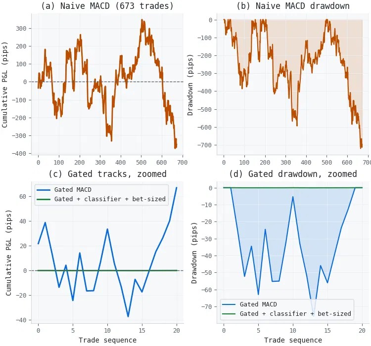
Figure 2. Four-panel illustration of the three-track out-of-sample comparison

• Panel (a): naive MACD's cumulative P&L across all 673 test-window trades, full scale.
• Panel (b): naive MACD's running drawdown, same scale.
• Panel (c): gated and gated-plus-sized cumulative P&L, zoomed to their own scale — 21 trades each, invisible on panel (a)'s axis.
• Panel (d): the same two tracks' running drawdown, zoomed.

Track	Trades	Total P&L (pips)	Max drawdown (pips)	Win rate
Naive MACD	673	−350.1	−720.3	51.0%
Gated MACD	21	+67.0	−76.0	61.9%
Gated + classifier + bet-sized	21	+0.1	−0.1	61.9%

Naive MACD loses money on the 17-month out-of-sample test window: −350.1 pips across 673 trades, an average of −0.52 pips per trade, with a win rate of 51.0% indistinguishable from a coin flip. This is the failure mode from Section 2 showing up as a bottom line on the test window, before any spread cost is even applied.

The gate's contribution here is not purely mechanical, which is the headline difference from a synthetic panel. Trade count falls 32× (673 → 21), which contributes to drawdown compression — though drawdown also depends on the sequence and size of losses, not trade count alone — and the average trade also flips sign and grows: −0.52 → +3.19 pips, with win rate rising to 61.9%.

That improvement should still be read cautiously. With only 21 gated trades, the 95% Wilson interval on the gated win rate is [41%, 79%], which comfortably contains 50%. The 21 gated trades are a subset of the 673 raw signals, not an independent sample, so a two-proportion test such as Fisher's exact test — which assumes independent groups — is not valid here and is not reported. The point estimate is encouraging and consistent with filtering the whipsaw trades documented in Section 2, but it is not statistically significant, and the +67.0-pip total is not robust to parameter selection on this small an event count.

The classifier layer tells a different, more clear-cut story. Its out-of-sample AUC on the test window is 0.500 — exactly chance — trained on 43 examples and evaluated on 21. This is a direct consequence of how strict the gate is on real data: 86 signals pass it across the entire seven-year history, 2.5% of the 3,392 raw crossovers, split roughly 17/43/21 across the gate-tuning, training, and test windows once the calendar-fraction split is applied. With min_samples_leaf=20 and 43 training rows, the Random Forest has almost no room to find a split that satisfies its own leaf-size floor. An AUC of exactly 0.500 means the model has no ranking power on the test set; it does not, by itself, tell us where the predicted probabilities sit — that would require an examination of the predict_proba distribution, which is not reported here. What bet_size_probability then produces from an uninformative classifier is a set of very small position sizes, and the gate's +67.0-pip result compresses to +0.1 pips. The classifier did not fail loudly; it failed by removing the gate's edge along with its risk.

This figure shows that the pipeline works end to end on real data: signal generation, gating, labeling, classifier training with sample weighting, bet sizing, and the three-way comparison. It also shows why a two-layer architecture can under-deliver: the second layer needs enough gated examples to learn from, and a strict gate can starve it. It does not demonstrate that the classifier or the twelve-feature panel are poorly designed in general; the honest conclusion is narrower, that this combination of gate strictness and training-window length left too little data for this layer, on this instrument, over this period. Before any of these numbers inform a trading decision, two things are still missing: spread costs applied to pnl_pips, and a rerun with either a looser gate, a longer or pooled training window, or a lower-capacity classifier sized to the sample the gate actually produces.

Discussion and Limitations

Six limitations are worth stating explicitly rather than leaving for the reader to infer:

• No transaction costs. The P&L series in Section 6 is gross; trade_pnl_pips returns raw pips per trade. The source data carries a real per-bar spread column that is not yet applied. Part 1 found that a mean-reversion filter's contribution to total P&L can be minimal even when its contribution to drawdown is substantial; naive MACD's 673 test-window trades make this article's naive track exactly the case where spread cost would matter most, and a strategy already losing 350 pips gross will only lose more net.
• Mid-price labeling. Mid-price is used for signals, features, triple-barrier labels, the gate objective, and classifier training. Real bid/ask data could flip marginal labels, change the gate's optimal parameters, and alter the RF training set — not just the final P&L.
• Small classifier sample. Forty-three training examples and 21 test examples are a direct consequence of a gate that passes only 2.5% of raw crossovers over seven years. The out-of-sample AUC of exactly 0.500 is the visible symptom: the classifier had too little data to learn from and too little room, given min_samples_leaf=20, to try. This is the most material limitation in this article, not a footnote to it.
• Gate optimization is in-sample for the gate. Optuna's 40-trial search over a 3-parameter space on the gate-opt window is a form of in-sample optimization, even though that window is held out from classifier training and from the final test period. The Wilson lower-bound objective penalizes small samples but does not correct for the fact of multiple parameter searches. No Bonferroni-style or deflated-Sharpe-style adjustment is applied. The gate's parameters should be re-derived on any new dataset before use.
• Potential weight leakage. get_event_weights is called on the full event set before the train/test split in the code as written. If uniqueness weights are computed globally, training weights may depend on test-period concurrency. The split should be applied before weight computation; the current ordering is flagged but not corrected in the excerpt shown.
• Untested parameter interaction. zero_line_required and confirm_bars can interact: a strict persistence requirement can make the zero-line flag close to redundant, or vice versa. The Optuna search treated them as independent, which the gate-opt window's signal density may not have been sufficient to fully disentangle.

One design tradeoff is worth stating as a considered choice rather than a default. hist_zero_crossings_20 counts the frequency of histogram sign changes in the trailing 20 bars; the gate's min_hist_atr condition floors the magnitude of the histogram at the signal bar. They measure different things — how often the histogram has been flipping versus how large it is right now — and the article does not equate them. Collapsing them into a single feature was considered and rejected: the gate needs a hard, auditable cutoff a trader can reason about before the fact, while the classifier benefits from the continuous count as one input among twelve, not the deciding one. Keeping them separate costs one feature's worth of correlation the Random Forest has to absorb, in exchange for a gate whose behavior does not depend on how the classifier happens to weight a shared feature.

Conclusion

MACD's signal-line crossover carries no explicit information about the magnitude or persistence of the momentum change that produced it — the crossover event alone, separate from the accompanying indicator values, is uninformative about what happens next — and a market that spends any material time ranging will feed the rule whipsaw trades indistinguishable, at entry, from genuine trend catches. On the 17-month out-of-sample test window, that failure mode costs the naive rule 350 pips gross across 673 trades. The Optuna-optimized regime gate built here — three parameters with no author-specified precedent in Appel's original work — turns that into a 21-trade track with a positive, though not statistically significant, average trade.

The Random Forest secondary classifier layered on top does not extend that result: with only 43 training examples, its out-of-sample AUC lands at exactly 0.500, and bet_size_probability faithfully shrinks the gate's edge to near zero along with its risk. The engineering layer worked; the machine-learning layer, on this instrument and this sample, had too little to learn from. A companion MQL5 article will address the execution-layer architecture that translates these Python outputs into a live trading system, following the two-EA pattern established in Part 1.

Attached Files

	File	Module	Description
1.	trading_strategies.py	afml.strategies	MACDStrategy: signal-line crossover primary model, alongside the shared BaseStrategy interface.
2.	macd_gate.py	article script	GateParams, apply_regime_gate, and optimize_regime_gate — the Optuna-optimized regime gate and its Wilson-lower-bound objective.
3.	macd_features.py	article script	build_macd_features — the twelve contextual features listed in Section 4.
4.	macd_pipeline.py	article script	Split bounds, labeling, classifier training, bet sizing, and the three-track backtest orchestration.
5.	triple_barrier.py, bet_sizing.py, ch10_snippets.py, optimized_concurrent.py, optimized_attribution.py, trading_session.py, filters.py, volatility.py, misc.py	afml	Minimal excerpt of the Blueprint Quant afml package — only the functions this article's code calls, not the complete package. Place the afml/ folder alongside the scripts above, or substitute your own afml installation if you already have the full package.

Further Reading

• López de Prado, M. (2018). Advances in Financial Machine Learning. John Wiley & Sons.
• Appel, G. (1979). The Moving Average Convergence-Divergence Trading Method.
• Wilder, J. W. (1978). New Concepts in Technical Trading Systems.