

Neural Networks in Trading: A Unified View of Space and Time (Global-Local Attention)
 79
79
 0
0

Introduction
Financial markets are a complex and dynamic system in which space and time are closely intertwined. Every price movement reflects not only the instantaneous balance of supply and demand, but also the traces of previous events, as well as the influence of related instruments, sectors, and even entire economies. Predicting the behavior of such a system using traditional methods has always been a highly complex task. Statistical models and classical neural networks performed reasonably well in short-term forecasting, but lost stability and accuracy when attempting to go beyond a few hours. The main problem was that temporal and spatial factors were considered separately. Attempts to combine them, however, led to an explosive increase in computational costs.
The Extralonger framework, which we began exploring in the previous article, offered a fundamentally different approach. Its authors were guided by the idea that space and time should be viewed as a single whole. This philosophy, which echoes Einstein's theory of relativity, was embodied in the Unified Spatial-Temporal Representation — a representation in which time series and spatial relationships are integrated without artificial separation. This solution led to a dramatic reduction in computational complexity. Where operations previously grew exponentially, Extralonger reduced them to quadratic dependencies. The practical results were impressive. Training accelerated hundreds of times, memory consumption was reduced manyfold, and, most importantly, it became possible to build forecasts spanning not just hours, but entire days and even weeks.
This opens up new opportunities for financial markets. Where traders and analysts have traditionally limited themselves to short-term assessments, there is now an opportunity to look ahead several trading sessions or predict market movements around the release of macroeconomic data and central bank decisions. Extralonger transforms a weekly forecast from an unattainable dream into a tool that can be put to practical use.
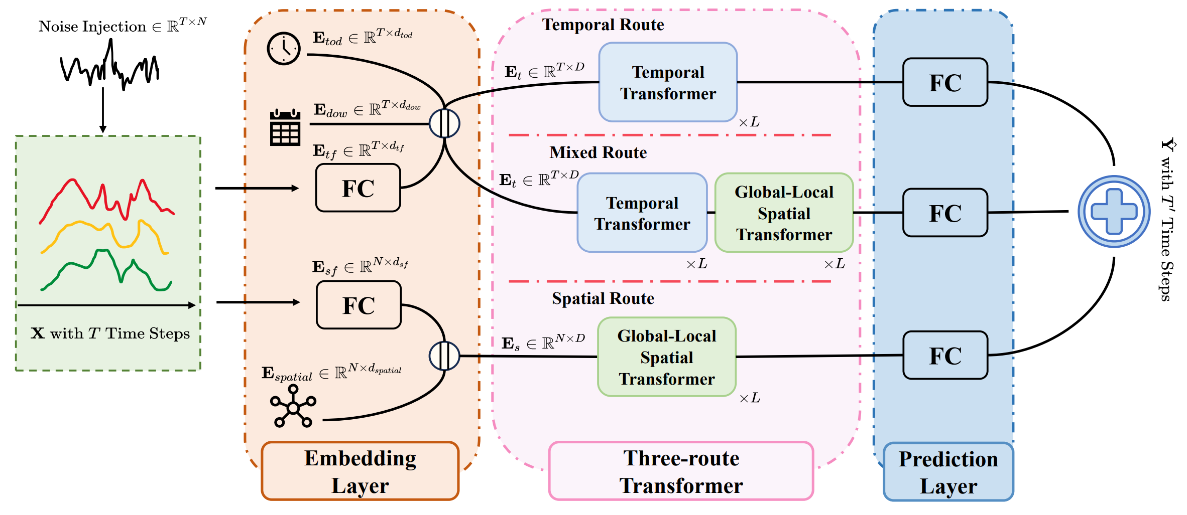
However, the framework's true power is revealed through its architecture. It is based on a three-branch Transformer, with each route responsible for a specific aspect of the analysis.
The temporal route can be compared to a macroeconomic analyst. He studies market rhythms, identifies cycles of growth and decline, and detects seasonality and recurring patterns. Using the Self-Attention mechanism, the model links distant segments of the time series. The current movement of the currency pair may be a continuation of the trend that began a month ago.
The spatial route serves as a specialist in cross-market relationships. In financial markets, no asset exists in isolation. Gold price movements are reflected in stock indices. The dollar exchange rate affects commodity markets. Bond yields, in turn, set the tone for stocks. Extralonger accounts for this through the Global-Local Spatial Transformer, which combines two perspectives: a global one, where each security is linked to all the others, and a local one, where the focus is on clusters of assets grouped by industry or region.
The mixed route most closely resembles the role of a portfolio manager. Its task is to combine temporal dynamics and spatial relationships into a single picture. As a result, the model perceives the market holistically. For the model, an increase in volatility in the technology sector, accompanied by changes in oil prices and fluctuations in interest rates, is not a set of random facts, but a signal that a major market scenario is forming.
The final forecast emerges at the point where the three routes intersect. Like an investment committee where each expert makes a contribution, Extralonger combines the conclusions of all participants into a weighted decision. As a result, the model gains not only local analytical depth and coverage of global connections, but also a holistic perception of market processes over time.
This design makes the framework particularly valuable for financial applications. It combines the depth of time-series analysis, broad coverage of cross-market relationships, and holistic perception. As a result, Extralonger can build robust forecasts where other models either lose accuracy or require excessive resources.
The author's visualization of the Extralonger framework is shown below.
In the practical section of the previous article, we took the first steps toward implementing the proposed approaches using MQL5. A spatial encoding module was developed to handle the interdependencies between instruments, and individual blocks of the OpenCL program for temporal encoding were also presented. These developments have become the foundation upon which we can build a fully fledged engineering version of the framework.
Today, we continue this work, moving further toward the practical implementation of the ideas behind Extralonger. Our goal is to gradually port the architecture proposed by the authors to the MQL5 environment, ensuring its viability with real financial data.
Temporal Embedding
We are continuing our work on developing algorithms for the Extralonger framework using MQL5. In the previous article, we took a detailed look at the kernels of the OpenCL program that add temporal embeddings to the input data. Now we move on to organizing this process on the main program side. To do this, we create a new CNeuronTempEmbedding object that inherits the basic functionality from the CNeuronBaseOCL class.
class CNeuronTempEmbedding    : public CNeuronBaseOCL
  {
protected:
   uint              iWindow;
   uint              iUnits;
   uint              aiEmbeddingDim[2];
   uint              aiFrames[2];
   uint              aiPeriod[2];
   CParams           caEmbeddings[2];
   //---
   virtual bool      ConcatByLabel(CNeuronBaseOCL *NeuronOCL, CBufferFloat *SecondInput);
   virtual bool      ConcatByLabelGrad(CNeuronBaseOCL *NeuronOCL, CBufferFloat *SecondInput);
   //---
   virtual bool      feedForward(CNeuronBaseOCL *NeuronOCL) override {return false;}
   virtual bool      feedForward(CNeuronBaseOCL *NeuronOCL, CBufferFloat *SecondInput) override;
   virtual bool      updateInputWeights(CNeuronBaseOCL *NeuronOCL) override;
   virtual bool      calcInputGradients(CNeuronBaseOCL *NeuronOCL) override {return false;}
   virtual bool      calcInputGradients(CNeuronBaseOCL *NeuronOCL,
                                        CBufferFloat *SecondInput,
                                        CBufferFloat *SecondGradient,
                                        ENUM_ACTIVATION SecondActivation = None
                                       ) override;

public:
                     CNeuronTempEmbedding(void) {};
                    ~CNeuronTempEmbedding(void) {};
   //---
   virtual bool      Init(uint numOutputs, uint myIndex, COpenCLMy *open_cl,
                          uint units, uint window,
                          uint embed_dim1, uint period1, uint frame1,
                          uint embed_dim2, uint period2, uint frame2,
                          ENUM_OPTIMIZATION optimization_type, uint batch);
   //---
   virtual int       Type(void)   const   {  return defNeuronTempEmbedding;   }
   //--- methods for working with files
   virtual bool      Save(int const file_handle) override;
   virtual bool      Load(int const file_handle) override;
   //---
   virtual bool      WeightsUpdate(CNeuronBaseOCL *source, float tau) override;
   virtual void      SetOpenCL(COpenCLMy *obj) override;
   virtual void      SetActivationFunction(ENUM_ACTIVATION value) override { };
  };
The main parameters of the object include the number of analyzed features iWindow, the sequence length iUnits, the embedding dimensions aiEmbeddingDim, the size of a single step iFrames, and the repetition periods aiPeriod. All of this is defined using arrays, which makes the object flexible and adaptable to different time scales of financial data.
The object structure is defined in the Init method, which is responsible for initializing all key parameters of the temporal encoding layer and its internal components.
bool CNeuronTempEmbedding::Init(uint numOutputs, uint myIndex, COpenCLMy *open_cl,
                                uint units, uint window,
                                uint embed_dim1, uint period1, uint frame1,
                                uint embed_dim2, uint period2, uint frame2,
                                ENUM_OPTIMIZATION optimization_type, uint batch)
  {
   if(!CNeuronBaseOCL::Init(numOutputs, myIndex, open_cl,
                            (window + embed_dim1 + embed_dim2)*units, optimization_type, batch))
      return false;
In the first step, the parent class CNeuronBaseOCL is initialized. This is where the layer's main characteristics are specified and the inherited interfaces are initialized. If the base initialization fails, the function returns false, preventing further creation of an invalid object.
Next, two caEmbeddings components are initialized to generate temporal embeddings for the data. Each embedding is created based on its own dimension (embed_dim1 and embed_dim2) and repetition period (period1 and period2). This allows the model to capture temporal patterns at different scales and depths of analysis, which is especially important when working with the dynamics of financial markets.
   if(!caEmbeddings[0].Init(0, 0, OpenCL, embed_dim1 * period1, optimization, iBatch))
      return false;
   if(!caEmbeddings[1].Init(0, 1, OpenCL, embed_dim2 * period2, optimization, iBatch))
      return false;
After the embedding components have been successfully initialized, the object's parameters are stored in internal variables. These parameters define the structure of the temporal layer and control how the neuron sees the market over time.
   iWindow = window;
   iUnits = units;
   aiEmbeddingDim[0] = embed_dim1;
   aiEmbeddingDim[1] = embed_dim2;
   aiFrames[0] = MathMax(1, frame1);
   aiFrames[1] = MathMax(1, frame2);
   aiPeriod[0] = period1;
   aiPeriod[1] = period2;
//---
   return true;
  }
Finally, the method returns true, confirming that a fully operational object has been successfully created.
The feedForward method implements forward signal propagation through the layer. First, it checks whether the object is in training mode (bTrain==true). If so, a separate forward pass is performed for each embedding component. This step allows us to construct a tensor of temporal features to capture patterns across different time scales. If even one embedding cannot be processed, the function returns false, preventing the further propagation of invalid data.
bool CNeuronTempEmbedding::feedForward(CNeuronBaseOCL *NeuronOCL, CBufferFloat *SecondInput)
  {
   if(bTrain)
      for(uint i = 0; i < caEmbeddings.Size(); i++)
         if(!caEmbeddings[i].FeedForward())
            return false;
//---
   return ConcatByLabel(NeuronOCL, SecondInput);
  }
After the successful forward pass of the embedding components, the data is merged using the ConcatByLabel method, which is a wrapper for the corresponding kernel of the OpenCL program. Here, the temporal features are carefully integrated with the input data. As a result, the object generates a processing-ready signal that combines historical data with current market observations, ensuring the model's accuracy and sensitivity to financial market dynamics.
As you can see, the forward pass method is implemented in a fairly simple and linear manner. Similarly, the backward pass and gradient update methods are straightforward and follow the logic of standard neural network training; therefore, for a deeper understanding, you can study how they work on your own. The complete source code for the CNeuronTempEmbedding class and all of its methods is provided in the attachment, which will allow you to examine in detail the implementation and integration of this object into the model's computational chain.
Attention Object
After preparing the temporal embeddings and integrating them with the input data, we move on to the next stage of our work — implementing the algorithms of the Global-Local Spatial Attention module. Before moving on to coding, it is important to discuss the approach proposed by the framework's authors.
The main idea is to combine the global attention characteristic of classical Self-Attention with the local focus implemented through an adjacency matrix. This approach is similar to the graph convolution methods we have encountered before, but in this case, it has been adapted to the spatiotemporal structure of the data.
The authors of the article do not provide detailed information on how the adjacency matrix was constructed. To fill this gap, we use the Significant Neighbors Sampling algorithm from the SAGDFN framework. It is used to create a sparse adjacency matrix, which significantly conserves computational resources while preserving the model's ability to account for significant local dependencies. It should be noted that this approach introduces certain nuances into the implementation of the process, since working with a sparse matrix requires careful handling of indices and compute threads.
OpenCL context-side implementation
When porting algorithms to an OpenCL program, we face two significant challenges that directly affect the speed and accuracy of market data analysis. The first is the sequential execution of Global- and Local-Attention, which reduces the model's overall performance and slows down the processing of large streams of historical quotes. The second challenge is even more subtle: how to coordinate the full Global-Attention threads with a sparse adjacency matrix so as not to lose important information about local relationships between price levels. How effectively the model can recognize complex market patterns depends directly on the quality of this configuration.
Solving both problems turned out to be surprisingly straightforward. In the spirit of multi-head attention, we distributed the computations across separate threads, allowing the model to analyze different aspects of market data simultaneously. Of course, this required branching the algorithm depending on the particular attention head. However, this approach made it possible to maintain the speed and accuracy of processing large historical time series, which is critical for the timely identification of market patterns.
After resolving the execution-architecture issues for Global- and Local-Attention within the parallel threads of a single kernel, it was time to move on to the practical implementation of the forward pass algorithm. We implemented it in the GlobalLocalAttention kernel. Each line here represents a step the model takes in analyzing historical data and identifying meaningful signals.
__kernel void GlobalLocalAttention(__global const float *q,
                                   __global const float2* kv,
                                   __global float *scores,
                                   __global const float* mask,
                                   __global const float* label,
                                   __global float *out,
                                   const int dimension,
                                   const int total_kv,
                                   const int total_mask
                                  )
  {
//--- init
   const int q_id = get_global_id(0);
   const int local_id = get_local_id(1);
   const int h_id = get_global_id(2);
   const int total_q = get_global_size(0);
   const int total_local = get_local_size(1);
   const int total_heads = get_global_size(2);
//---
   __local float temp[LOCAL_ARRAY_SIZE];
The kernel receives all the key data:
- query vectors q — our current market queries,
- key-value pairs kv — historical patterns and their outcomes,
- a mask and labels for local constraints,
- parameters for the dimensions of the feature space and data volumes.
In the kernel body, the model first determines which entity is which in the three-dimensional problem space:
- q_id is a specific query;
- local_id is a thread within a group that, depending on the attention head, points to either a key-query pair or a position in a sparse adjacency matrix:
- h_id is an attention head that analyzes a specific aspect of the market.
A local array serves as a temporary buffer for intermediate calculations, much like a trader's desk where all current results are gathered before the final evaluation.
Next, we determine the memory offset of the query being analyzed — it is like finding the right bar on a chart to compare it with historical price movements.
int shift_q = RCtoFlat(h_id, 0, total_heads, dimension, q_id);
We then set up a branch in the algorithm: even attention heads provide a global view of the market, where key patterns are assessed across the entire historical dataset, while odd attention heads provide a local view.
For even attention heads, we calculate the positions of the keys and the corresponding attention coefficients. It is like marking all past support and resistance levels on the chart for the current query.
   if(h_id % 2 == 0)
     {
      const int shift_kv = RCtoFlat(h_id, 0, total_heads, dimension, local_id);
      const int shift_s = RCtoFlat(h_id / 2, local_id, total_heads / 2, total_kv + total_mask, q_id);
      float score = 0;
      if(local_id < total_kv)
        {
         //---
         for(int d = 0; d < dimension; d++)
            score += IsNaNOrInf(q[shift_q + d] * kv[shift_kv + d].s0, 0);
        }
      else
         score = MIN_VALUE;
      //--- norm score
      score = LocalSoftMax(score, 1, temp);
      if(local_id < total_kv)
         scores[shift_s] = score;
We calculate the correlation between the current query and historical data. If a thread does not participate in the calculation, we assign it the minimum value so it does not distort the picture, like inactive traders in the market. After that, we normalize the weight of each pattern. It's like weighing the importance of signals: some price levels have a stronger impact, while others are barely taken into account.
Final assembly of the output: we multiply the historical values by their weights and sum them.
      //--- out
      for(int d = 0; d < dimension; d++)
        {
         float val = (local_id < total_kv ? kv[shift_kv + d].s1 * score : 0);
         val = LocalSum(val, 1, temp);
         if(local_id == 0)
            out[shift_q + d] = val;
        }
     }
The output is a signal for the current query, ready for analysis or use in a trading strategy.
The second branch of the algorithm processes local connections using the corresponding mask. Here, we are essentially working with a sparse adjacency matrix, in which many elements are either missing or irrelevant to the current analysis.
The algorithm begins by checking whether a connection exists for the current local element. The local variable kv_id points to the actual key with which the attention coefficient must be computed. If kv_id is less than 0, it means there is no corresponding element in the sparse matrix, and the thread is skipped. The m mask further filters out invalid connections.
   else
     {
      int kv_id = -1;
      float score = 0;
      int shift_kv = -1;
      float m = 0;
      if(local_id < total_mask)
        {
         const int shift_s = RCtoFlat(h_id / 2, total_kv + local_id, total_heads / 2,
                                                        total_kv + total_mask, q_id);
         const int l = RCtoFlat(q_id, local_id, total_q, total_mask, 0);
         kv_id = IsNaNOrInf(label[l], -1);
         m = IsNaNOrInf(mask[l], 0);
         shift_kv = RCtoFlat(h_id, 0, total_heads, dimension, kv_id);
         if(kv_id >= 0)
            for(int d = 0; d < dimension; d++)
               score += IsNaNOrInf(q[shift_q + d] * kv[shift_kv + d].s0, 0);
         else
            score = MIN_VALUE;
        }
      else
         score = MIN_VALUE;
      //--- norm score
      score = LocalSoftMax(score * m, 1, temp);
      if(local_id < total_mask)
         scores[shift_s] = score;
Only existing local connections are used in the calculation of attention coefficients; the rest are assigned a minimum value. This ensures that the sparse structure does not contaminate the result, and that the model focuses exclusively on relevant local patterns.
SoftMax normalization takes the mask into account so that the total probability is distributed only across actual local elements.
Finally, we generate the output for the query, taking into account only those local patterns that are actually present in the sparse matrix.
      //--- out
      for(int d = 0; d < dimension; d++)
        {
         float val = (kv_id >= 0 ? IsNaNOrInf(kv[shift_kv + d].s1, 0) * score : 0);
         val = LocalSum(val, 1, temp);
         if(local_id == 0)
            out[shift_q + d] = val;
        }
     }
  }
The use of a sparse matrix makes it impossible to have a simple, universal algorithm for all attention heads. The global attention head operates on a dense matrix — all elements are present, and the computations are straightforward. The local attention head operates on a sparse structure — many connections are missing, so mask and label checks, NaN/Inf filtering, and separate summation logic are required. Therefore, within a single kernel, we had to implement two separate algorithms, each optimized for its own data type: one for a dense global matrix, and the other for a sparse local matrix.
Once the forward pass had been implemented, we faced a much more challenging task — distributing the error gradients. The GlobalLocalAttentionGrad kernel acts here like an experienced trader who keeps an eye on both the big picture and local patterns at the same time. Each thread within the kernel is like a separate analyst who is assigned their own section of the chart. However, this is not a narrow slice of work.
The interpretation of global_id here varies depending on the specific stage. It can point to Query, Key, or Value. Its role changes at each stage and indicates the object for which the error gradient is being computed. Similarly, the functionality of local_id changes; it defines the thread within a group, much like a trader viewing multiple timeframes. And h_id determines the attention head — that is, the aspect of the market on which the analyst is focusing.
All these indices form an observation network, allowing gradients to be distributed precisely, as if we were dividing our attention among different quotes so that no detail goes unnoticed.
__kernel void GlobalLocalAttentionGrad(__global const float *q,
                                       __global float *q_gr,
                                       __global const float *kv,
                                       __global float *kv_gr,
                                       __global float *scores,
                                       __global const float *mask,
                                       __global const float *mask_gr,
                                       __global const float *label,
                                       __global float *out_gr,
                                       const int dimension,
                                       const int total_q,
                                       const int total_kv,
                                       const int total_mask
                                      )
  {
//--- init
   const int global_id = get_global_id(0);
   const int local_id = get_local_id(1);
   const int h_id = get_global_id(2);
   const int total_global = get_global_size(0);
   const int total_local = get_local_size(1);
   const int total_heads = get_global_size(2);
//---
   __local float temp[LOCAL_ARRAY_SIZE];
For even attention heads, which work with a global dense matrix, the process is similar to market analysis based on complete historical data. First, the gradients for Value are computed: each thread accumulates the effect of its position on the overall result by summing it via LocalSum. It is similar to how a trader aggregates signals from all historical candlesticks to identify the overall trend.
   if(h_id % 2 == 0)
     {
      //--- Value Gradient global_id -> v_id, local_id -> q_id
      for(int d = 0; d < dimension; d++)
        {
         const int shift_v = RCtoFlat(h_id, 2 * d + 1, total_heads, 2 * dimension, global_id);
         float grad = 0;
         for(int q_id = local_id; q_id < total_q; q_id += total_local)
           {
            int shift_s = RCtoFlat(h_id / 2, global_id, total_heads / 2, total_kv + total_mask, q_id);
            int shift_q = RCtoFlat(h_id, d, total_heads, dimension, q_id);
            grad += IsNaNOrInf(scores[shift_s] * out_gr[shift_q], 0);
           }
         grad = LocalSum(grad, 1, temp);
         kv_gr[shift_v] = grad;
        }
Next, the gradients for Query are computed. It is important to take SoftMax normalization into account here — just as an analyst evaluates the significance of each signal relative to all the others, so that no noise distorts the picture. Query gradients are carefully summed across local threads and written to q_gr.
      //--- Query Gradient global_id -> q_id, local_id -> k_id/v_id
      if(global_id < total_q)
        {
         //--- 1. Score grad
         float grad_s = 0;
         const int shift_v = RCtoFlat(h_id, 1, total_heads, 2 * dimension, local_id);
         const int shift_s = RCtoFlat(h_id / 2, local_id, total_heads / 2,
                                          total_kv + total_mask, global_id);
         int shift_q = RCtoFlat(h_id, 0, total_heads, dimension, global_id);
         if(local_id < total_kv)
            for(int d = 0; d < dimension; d++)
               grad_s += IsNaNOrInf(kv[shift_v + 2 * d] * out_gr[shift_q + d], 0);
         //--- 2. SoftMax grad
         grad_s = LocalSoftMaxGrad(scores[shift_s], grad_s, 1, temp);
         //--- 3. Query grad
         const int shift_k = shift_v - 1;
         for(int d = 0; d < dimension; d++)
           {
            float grad = 0;
            if(local_id < total_kv)
               grad = kv[shift_k + 2 * d] * grad_s;
            grad = LocalSum(grad, 1, temp);
            if(local_id == 0)
               q_gr[shift_q + d] = grad;
           }
        }
Key obtains the final gradients by summing the contributions from all queries.
      //--- Key Gradient global_id -> k_id, local_id -> score_id/v_id/dimension
      if(global_id < total_kv)
        {
         float grad = 0;
         for(int q_id = 0; q_id < total_q; q_id++)
           {
            //--- 1. Score grad local_id -> score_id/v_id
            float grad_s = 0;
            const int shift_v = RCtoFlat(h_id, 1, total_heads, 2 * dimension, local_id);
            const int shift_s = RCtoFlat(h_id / 2, local_id, total_heads / 2,
                                                total_kv + total_mask, q_id);
            int shift_q = RCtoFlat(h_id, 0, total_heads, dimension, q_id);
            if(local_id < total_kv)
               for(int d = 0; d < dimension; d++)
                  grad_s += IsNaNOrInf(kv[shift_v + 2 * d] * out_gr[shift_q + d], 0);
            //--- 2. SoftMax grad
            grad_s = LocalSoftMaxGrad(scores[shift_s], grad_s, 1, temp);
            BarrierLoc;
            if(global_id == local_id)
               temp[0] = grad_s;
            BarrierLoc;
            grad_s = temp[0];
            //--- 3. Key grad local_id -> dimension
            shift_q = RCtoFlat(h_id, local_id, total_heads, dimension, q_id);
            if(local_id < dimension)
               grad += IsNaNOrInf(q[shift_q] * grad_s, 0);
           }
         const int shift_k = RCtoFlat(h_id, 2 * local_id, total_heads, 2 * dimension, global_id);
         if(local_id < dimension)
            kv_gr[shift_k] = IsNaNOrInf(grad);
        }
     }
For the global matrix, the process runs smoothly because all the data is present, and the algorithm can distribute the gradients in parallel.
Odd attention heads that work with a local sparse matrix require true trader-like meticulousness from the kernel. As in the algorithm presented above, we first loop over and sum the gradients for Value from all Query entries. But here, for each one, we first check whether a connection exists via the mask and labels. If there is no connection, or if the mask prohibits the use of the element, the Query thread is skipped.
   else
     {
      //--- Value Gradient global_id -> v_id, local_id -> mask_index/dimension
      if(global_id < total_kv)
        {
         float grad = 0;
         for(int q_id = 0; q_id < total_q; q_id++)
           {
            //--- 1. kv_id
            int kv_id = -1;
            float m = 0;
            const int l = RCtoFlat(q_id, local_id, total_q, total_mask, 0);
            const int shift_s = RCtoFlat(h_id / 2, total_kv + local_id, total_heads / 2,
                                                           total_kv + total_mask, q_id);
            //--- Check whether current Value is used
            if(local_id < total_mask)
               kv_id = (int)label[l];
            if(local_id == 0)
               temp[0] = 0;
            BarrierLoc;
            if(kv_id == global_id)
               temp[0] = scores[shift_s];
            BarrierLoc;
            if(temp[0] == 0)
               continue;
The Value gradient is calculated only for existing elements. The attention coefficient is multiplied by the corresponding output gradient and accumulated.
            //--- Value grad
            int shift_q = RCtoFlat(h_id, local_id, total_heads, dimension, q_id);
            if(local_id < dimension)
               grad += IsNaNOrInf(temp[0] * out_gr[shift_q], 0);
           }
         const int shift_v = RCtoFlat(h_id, 2 * local_id + 1, total_heads, 2 * dimension, global_id);
         if(local_id < dimension)
            kv_gr[shift_v] = IsNaNOrInf(grad, 0);
        }
Query gradients are formed taking SoftMax and the mask into account, which makes it possible to filter out extraneous signals, just as a trader ignores noisy bars and false patterns.
      //--- Query Gradient global_id -> q_id, local_id -> mask label
      if(global_id < total_q)
        {
         //--- 1. kv_id;
         int kv_id = -1;
         float m = 0;
         const int l = RCtoFlat(global_id, local_id, total_q, total_mask, 0);
         if(local_id < total_mask)
           {
            kv_id = (int)IsNaNOrInf(label[l], -1);
            m = IsNaNOrInf(mask[l], 0);
           }
         //--- 2. Score grad
         float grad_s = 0;
         const int shift_v = RCtoFlat(h_id, 1, total_heads, 2 * dimension, kv_id);
         const int shift_s = RCtoFlat(h_id / 2, total_kv + local_id, total_heads / 2,
                                                   total_kv + total_mask, global_id);
         int shift_q = RCtoFlat(h_id, 0, total_heads, dimension, global_id);
         if(local_id < total_mask)
            for(int d = 0; d < dimension; d++)
               grad_s += IsNaNOrInf(kv[shift_v + 2 * d] * out_gr[shift_q + d], 0);
         //--- 3. SoftMax grad
         float score = IsNaNOrInf(scores[shift_s], 0);
         grad_s = LocalSoftMaxGrad(scores[shift_s], grad_s, 1, temp);
         mask_gr[l] = IsNaNOrInf(grad_s * score, 0);
         grad_s *= m;
         //--- 4. Query grad
         const int shift_k = shift_v - 1;
         for(int d = 0; d < dimension; d++)
           {
            float grad = 0;
            if(local_id < total_mask)
               grad = kv[shift_k + 2 * d] * grad_s;
            grad = LocalSum(grad, 1, temp);
            if(local_id == 0)
               q_gr[shift_q + d] = grad;
           }
        }
Key gradients are accumulated only for those queries that actually have a connection to the key, and thread synchronization via BarrierLoc ensures that no signal is lost. It is as if an analyst were cross-checking colleagues’ results before making the final trade entry. Each computation accurately reflects the actual distribution of influence in the local sparse matrix and prevents gradient contamination by unnecessary data.
      //--- Key Gradient global_id -> k_id, local_id -> score_id/v_id/dimension
      if(global_id < total_kv)
        {
         float grad = 0;
         for(int q_id = 0; q_id < total_q; q_id++)
           {
            //--- 1. kv_id;
            int kv_id = -1;
            float m = 0;
            const int l = RCtoFlat(global_id, local_id, total_q, total_mask, 0);
            if(local_id < total_mask)
              {
               kv_id = (int)label[l];
               if(kv_id == global_id)
                  m = mask[l];
              }
            m = LocalSum(m, 1, temp);
            if(m == 0)
               continue;
            //--- 2. Score grad local_id -> score_id/v_id
            float grad_s = 0;
            const int shift_v = RCtoFlat(h_id, 1, total_heads, 2 * dimension, kv_id);
            const int shift_s = RCtoFlat(h_id / 2, total_kv + local_id, total_heads / 2,
                                                           total_kv + total_mask, q_id);
            int shift_q = RCtoFlat(h_id, 0, total_heads, dimension, q_id);
            if(local_id < total_mask)
               for(int d = 0; d < dimension; d++)
                  grad_s += IsNaNOrInf(kv[shift_v + 2 * d] * out_gr[shift_q + d], 0);
            //--- 3. SoftMax grad
            grad_s = LocalSoftMaxGrad(scores[shift_s], grad_s, 1, temp);
            BarrierLoc;
            if(global_id == local_id)
               temp[0] = grad_s * m;
            BarrierLoc;
            grad_s = temp[0];
            //--- 4. Key grad local_id -> dimension
            shift_q = RCtoFlat(h_id, local_id, total_heads, dimension, q_id);
            if(local_id < dimension)
               grad += IsNaNOrInf(q[shift_q] * grad_s, 0);
           }
         const int shift_k = RCtoFlat(h_id, 2 * local_id, total_heads, 2 * dimension, global_id);
         if(local_id < dimension)
            kv_gr[shift_k] = IsNaNOrInf(grad);
        }
     }
  }
Two logically distinct algorithms are implemented within a single kernel because the global and local matrices require fundamentally different approaches. A global dense matrix allows gradients to be computed directly for all elements, as if the trader could see the entire market at a glance. A local sparse matrix requires careful filtering, synchronization, and summation only over existing connections. Similarly to a trader who carefully checks every important signal on a limited section of the chart. This separation ensures the correct and efficient distribution of gradients when training the model on large historical time series, where dense global dependencies and sparse local correlations coexist.
Every action of the kernel is like a separate step taken by a trader. Checking the mask and labels is similar to selecting truly significant price levels. Filtering NaN and Inf means ignoring noisy data. Summation via LocalSum and thread synchronization correspond to coordinating analysts so as not to miss important signals. As a result, the model obtains accurate gradients for Value, Query, and Key, which allows it to learn from historical data, recognize significant market patterns, and minimize the prediction error. The kernel transforms abstract computations into a dynamic market analysis process, where each gradient operation reflects the analyst's actual attention and actions, ensuring accurate and stable training.
The complete kernel code is included in the attachment.
Implementation in the Main Program
In the main program, the Global-Local Spatial Attention algorithm is neatly implemented as a new object, CNeuronGlobalLocalAttention, which inherits the functionality of the multi-head feed-forward structure CNeuronMHFeedForward. This object combines several key components, each of which plays a strictly defined role in building attention.
class CNeuronGlobalLocalAttention   :  public CNeuronMHFeedForward
  {
protected:
   CNeuronSNSMHAttention   cMask;
   CNeuronConvOCL          cQ;
   CNeuronConvOCL          cKV;
   CNeuronBaseOCL          cScore;
   CNeuronBaseOCL          cMHAttention;
   CNeuronConvOCL          cW0;
   CNeuronBaseOCL          cResidual;
   //---
   virtual bool      GlobalLocalAttention(void);
   virtual bool      GlobalLocalAttentionGrad(void);
   //---
   virtual bool      feedForward(CNeuronBaseOCL *NeuronOCL) override;
   virtual bool      updateInputWeights(CNeuronBaseOCL *NeuronOCL) override;
   virtual bool      calcInputGradients(CNeuronBaseOCL *NeuronOCL) override;

public:
                     CNeuronGlobalLocalAttention(void) {};
                    ~CNeuronGlobalLocalAttention(void) {};
   //---
   virtual bool      Init(uint numOutputs, uint myIndex, COpenCLMy *open_cl,
                          uint units, uint window, uint dimension_k,
                          uint heads, uint m_units, float sparse,
                          ENUM_OPTIMIZATION optimization_type, uint batch);
   //---
   virtual int       Type(void)   const   {  return defNeuronGlobalLocalAttention;   }
   //--- methods for working with files
   virtual bool      Save(int const file_handle) override;
   virtual bool      Load(int const file_handle) override;
   //---
   virtual bool      WeightsUpdate(CNeuronBaseOCL *source, float tau) override;
   virtual void      SetOpenCL(COpenCLMy *obj) override;
   virtual void      SetActivationFunction(ENUM_ACTIVATION value) override { };
  };
Inside the class is the cMask object, which is responsible for managing local connection masks, allowing the class to correctly handle a sparse matrix and filter out irrelevant local patterns. Two convolution objects, cQ and cKV, perform transformations on queries and key-value pairs, respectively, preparing the data for calculating attention coefficients. The cScore element accumulates the scores, while cMHAttention collects the results of multi-head attention, combining global and local components. Finally, cW0 and cResidual are responsible for the linear transformation and the addition of the residual connection, ensuring the stability and correctness of the output signal updates. The functionality of the FeedForward block is implemented by the parent class.
The Init method is responsible for fully initializing the neuron and sets all the key parameters for the Global-Local Spatial Attention algorithm. First, the base class CNeuronMHFeedForward is initialized. All the main parameters of the object are specified here.
bool CNeuronGlobalLocalAttention::Init(uint numOutputs, uint myIndex, COpenCLMy *open_cl,
                                       uint units, uint window, uint dimension_k,
                                       uint heads, uint m_units, float sparse,
                                       ENUM_OPTIMIZATION optimization_type, uint batch)
  {
   if(!CNeuronMHFeedForward::Init(numOutputs, myIndex, open_cl, window, 2 * window, units,
                                                      1, heads, optimization_type, batch))
      return false;
   activation = None;
If something goes wrong at this stage, the trading session does not start: the object is not initialized, thereby preventing any incorrect calculations.
Next, we disable the activation function, as if the trader had decided to trade without emotional filters, relying entirely on direct market signals.
First up is cMask. It manages local masks, filtering sparse patterns so that the trader is not distracted by insignificant signals. With its help, the model understands which local connections are important and which can be ignored.
   int index = 0;
   if(!cMask.Init(0, index, OpenCL, units, window, heads, m_units, sparse, optimization, iBatch))
      return false;
Next, cQ and cKV are generated, transforming raw data into meaningful analytical signals. cQ processes queries, much like a trader assesses current market positions, while cKV accumulates keys and values, much like a trader gathers information about past candlesticks, support levels, and resistance levels. For both blocks, the activation function is disabled so that the analysis lines remain clean and linear, without distortion.
   index++;
   if(!cQ.Init(0, index, OpenCL, window, window, 2 * dimension_k * heads, units, 1,
                                                             optimization, iBatch))
      return false;
   cQ.SetActivationFunction(None);
   index++;
   if(!cKV.Init(0, index, OpenCL, window, window, 4 * dimension_k * heads, units, 1,
                                                              optimization, iBatch))
      return false;
   cKV.SetActivationFunction(None);
Next, cScore is activated, which aggregates the received scores — similar to how a trader combines signals from all indicators to determine where to take a position.
   index++;
   if(!cScore.Init(0, index, OpenCL, (units + m_units)*units * heads, optimization, iBatch))
      return false;
   cScore.SetActivationFunction(None);
   index++;
   if(!cMHAttention.Init(0, index, OpenCL, 2 * dimension_k * heads * units, optimization, iBatch))
      return false;
   cMHAttention.SetActivationFunction(None);
Based on these scores, cMHAttention, a multi-head attention mechanism, distributes resources among different instruments and time intervals. Just as an experienced analyst decides what to focus on most in the current market situation.
The chain is completed by cW0 and cResidual. The first performs a linear transformation of the signals, much like a trader adjusts calculations to account for the current market volume and liquidity.
   index++;
   if(!cW0.Init(0, index, OpenCL, 2 * dimension_k * heads, 2 * dimension_k * heads,
                                           window, units, 1, optimization, iBatch))
      return false;
   cW0.SetActivationFunction(None);
   index++;
   if(!cResidual.Init(0, index, OpenCL, Neurons(), optimization, iBatch))
      return false;
   cResidual.SetActivationFunction(None);
//---
   return true;
  }
The second adds a residual connection, ensuring that information about previous training steps is not lost and that the signal remains stable — much like checking positions from previous trades before opening a new one.
Each block is assigned a unique index and parameters, is linked to the OpenCL context, and is ready to work together with the others. It all resembles a well-coordinated team of traders and analysts: one filters signals, another assesses trends, a third accumulates the results, and a fourth allocates attention among the instruments. As a result, once initialization is complete, the object is fully operational and capable of simultaneously analyzing global and local market patterns, filtering out noise, and making accurate decisions based on historical data.
Once the object has been initialized and all blocks have been configured, the forward pass begins — the point at which the model actually observes the market and generates its forecasts. The feedForward method defines a clear sequence of actions in which each component performs a strictly defined role, and the data passes through the entire chain of transformations, resembling the work of a well-coordinated team of traders.
bool CNeuronGlobalLocalAttention::feedForward(CNeuronBaseOCL *NeuronOCL)
  {
   if(!cMask.FeedForward(NeuronOCL))
      return false;
First, cMask is activated, checking and filtering local connections. It is like a trader carefully selecting only those signals that truly matter, ignoring noisy or missing patterns. If something goes wrong here, further analysis is impossible — the model will not generate a forecast based on incorrect data.
Next, cQ and cKV are executed in sequence. The first processes queries, preparing them for comparison with the keys, just as an analyst assesses current market positions and compiles a list of potential entry points.
   if(!cQ.FeedForward(NeuronOCL))
      return false;
   if(!cKV.FeedForward(NeuronOCL))
      return false;
The second one accumulates keys and values, as if compiling a history of quotes and trading volumes for each instrument, thereby creating a basis for assessing the impact of each signal.
After the preparatory phase is successfully completed, the GlobalLocalAttention wrapper method is called, which manages the process of queuing the kernel of the same name that executes the main algorithm within the OpenCL context.
   if(!GlobalLocalAttention())
      return false;
Here, queries and keys are combined into global and local attention. The magic of the model unfolds: each pattern is evaluated taking into account all relevant connections — both sparse and dense — and the contributions are carefully summed across all attention heads.
This stage is similar to the moment when a trader compares current signals with historical data and decides which positions deserve the most attention.
Next, cW0 is executed, which applies a linear transformation to the results of multi-head attention. This can be thought of as adjusting the signals to account for market size, liquidity, and the weight of each pattern.
   if(!cW0.FeedForward(cMHAttention.AsObject()))
      return false;
   if(!SumAndNormilize(NeuronOCL.getOutput(), cW0.getOutput(), cResidual.getOutput(),
                       cW0.GetFilters(), true, 0, 0, 0, cW0.GetUnits()))
      return false;
//---
   return CNeuronMHFeedForward::feedForward(cResidual.AsObject());
  }
After that, the data is passed through SumAndNormalize. It sums the outputs of the linear block and the residual connection, and then normalizes them. This step ensures that the signal remains stable and scalable — as if the trader had combined the findings of several analysts, verified their consistency, and assessed the overall strength of the signal before making a decision.
Finally, the updated signal is passed to the method of the same name in the parent class CNeuronMHFeedForward, which completes the forward pass by executing the functionality of the FeedForward block and integrating the results into the overall model structure.
Thus, the entire forward pass process can be viewed as a sequential market analysis in which each block performs a specific function: filtering, evaluating, accumulating, adjusting, and summing data, thereby ensuring the accuracy and consistency of forecasts.
Once the model has successfully completed a forward pass and generated a prediction, the training phase begins — the point at which the neuron evaluates how accurately it performed and adjusts its internal parameters. The calcInputGradients method is responsible for this evaluation and for distributing the quantified influence of each model component on the final result.
bool CNeuronGlobalLocalAttention::calcInputGradients(CNeuronBaseOCL *NeuronOCL)
  {
   if(!NeuronOCL)
      return false;
   if(!CNeuronMHFeedForward::calcInputGradients(cResidual.AsObject());)
      return false;
First, the validity of the received pointer to the NeuronOCL input data object is verified. If the object is missing, further calculations are impossible — just as if a trader were trying to analyze data without a chart or quotes.
Next, the method of the same name in the parent class is called, which initiates the process of backpropagating gradients down to the residual connection object.
Next, the DeActivation method is called for the cW0 block, where the obtained gradients are adjusted based on the activation function of the linear layer. This is similar to how an analyst takes into account the impact of each indicator on the final decision by filtering and normalizing the signals.
   if(!DeActivation(cW0.getOutput(), cW0.getGradient(), cResidual.getGradient(), cW0.Activation()))
      return false;
The gradients are then passed to cMHAttention, where the influence of each multi-head attention pattern is accumulated.
   if(!cMHAttention.CalcHiddenGradients(cW0.AsObject()))
      return false;
   if(!GlobalLocalAttentionGrad())
      return false;
At this stage, GlobalLocalAttentionGrad is called, which ensures the precise distribution of gradients between the global and local matrices, taking into account sparse and dense connections — much like a trader assesses the contribution of each candlestick and each support level to the overall trend. And the gradients are carefully propagated to the cQ and cKV blocks.
Next, we need to collect the error gradients at the input data level from all information streams. And we have four of them. First, we propagate the gradients down from cQ.
   if(!NeuronOCL.CalcHiddenGradients(cQ.AsObject()))
      return false;
We sum the resulting values with the gradients of the residual connection paths, but first we adjust the latter according to the activation function of the input data layer.
   if(!DeActivation(cResidual.getOutput(), cResidual.getGradient(),
                    cResidual.getGradient(), NeuronOCL.Activation()))
      return false;
   if(!SumAndNormilize(NeuronOCL.getGradient(), cResidual.getGradient(), cResidual.getGradient(),
                       cW0.GetFilters(), false, 0, 0, 0, cW0.GetUnits()))
      return false;
The next step involves processing the cKV gradients and then adding them to the previously accumulated data.
   if(!NeuronOCL.CalcHiddenGradients(cKV.AsObject()))
      return false;
   if(!SumAndNormilize(NeuronOCL.getGradient(), cResidual.getGradient(), cResidual.getGradient(),
                       cW0.GetFilters(), false, 0, 0, 0, cW0.GetUnits()))
      return false;
Last in order, but not in importance, we propagate the gradients of the local masks cMask downward. We also sum their influence with the data accumulated earlier.
   if(!NeuronOCL.CalcHiddenGradients(cMask.AsObject()))
      return false;
   if(!SumAndNormilize(NeuronOCL.getGradient(), cResidual.getGradient(), NeuronOCL.getGradient(),
                       cW0.GetFilters(), false, 0, 0, 0, cW0.GetUnits()))
      return false;
//---
   return true;
  }
As a result, the calcInputGradients method provides a comprehensive and detailed assessment of the impact of all model components — from global and local attention heads to queries, keys, values, and masks. Each block receives quantitative feedback, allowing the model to update its weights correctly, minimize error, and improve the accuracy of its forecasts. This process transforms abstract gradient calculations into a concrete assessment of the importance of each element in the system, making the training process as transparent and controllable as possible.
Once the model has estimated the impact of each component through gradient backpropagation, it is time to take action — adjust the internal parameters and adapt the model to real-world market data. The updateInputWeights method performs exactly this task.
bool CNeuronGlobalLocalAttention::updateInputWeights(CNeuronBaseOCL *NeuronOCL)
  {
   if(!cMask.UpdateInputWeights(NeuronOCL))
      return false;
   if(!cQ.UpdateInputWeights(NeuronOCL))
      return false;
   if(!cKV.UpdateInputWeights(NeuronOCL))
      return false;
   if(!cW0.UpdateInputWeights(cMHAttention.AsObject()))
      return false;
//---
   return CNeuronMHFeedForward::updateInputWeights(cResidual.AsObject());
  }
The algorithm behind the method is actually very straightforward — it sequentially delegates control to internal components that contain the trainable parameters. First, the weights of the local masks cMask are updated; then the parameters of the queries cQ and keys/values cKV are adjusted. After that, the weights of the linear transformation cW0 are updated. At the end, the parameters of the parent class are adjusted.
Each step is a simple yet important process: the model adjusts its parameters to assess the market more accurately and generate forecasts, while all components work in unison, like a team of traders following a unified strategy.
We have done a significant amount of work and successfully completed numerous tasks. Now is the perfect time to take a short break, catch your breath, and reflect on the results. In the next article, with renewed energy and a fresh perspective, we will continue our work and bring it to its logical conclusion.
Conclusion
We have come a long way: each block of the Global-Local Spatial Attention algorithm has been carefully integrated and arranged into a single computational pipeline. The forward pass, gradient distribution, and model parameter updates — all of this resembled the work of an experienced trader who filters signals, assesses the impact of each instrument, and adjusts positions to achieve the best possible result.
The approach implemented in MQL5 demonstrated how complex attention algorithms can be adapted for practical use, transforming abstract computations into accurate and controllable forecasts. Each block of the model, acting as an independent analyst, contributed to the final decision, ensuring the flexibility, robustness, and scalability of the entire system.
The next stage will serve as the final test of our work: we will bring the model to its logical conclusion, test it using real market data, and evaluate the practical effectiveness of the proposed framework.
References
- Extralonger: Toward a Unified Perspective of Spatial-Temporal Factors for Extra-Long-Term Traffic Forecasting
- Other articles in this series
Files used in the article
| # | Name | Type | Description |
|---|---|---|---|
| 1 | Study.mq5 | Expert Advisor | Expert Advisor for offline model training |
| 2 | StudyOnline.mq5 | Expert Advisor | Expert Advisor for online model training |
| 3 | Test.mq5 | Expert Advisor | Expert Advisor for model testing |
| 4 | Trajectory.mqh | Class library | Structure for describing the system state and model architecture |
| 5 | NeuroNet.mqh | Class library | Class library for building a neural network |
| 6 | NeuroNet.cl | Library | Code library for the OpenCL program |
Translated from Russian by MetaQuotes Ltd.
Original article: https://www.mql5.com/ru/articles/19538
Warning: All rights to these materials are reserved by MetaQuotes Ltd. Copying or reprinting of these materials in whole or in part is prohibited.
This article was written by a user of the site and reflects their personal views. MetaQuotes Ltd is not responsible for the accuracy of the information presented, nor for any consequences resulting from the use of the solutions, strategies or recommendations described.

 Encoding Candlestick Patterns (Part 5): Expanding Taxonomy of Candlestick for General Pattern Frequency Analysis
 Competitive Swarm Optimizer (CSO)
 From Deal History to Hazard Curves: Survival Analysis Applied To Strategies
 Working with ONNX Models in MQL5 (Part 2): Drawing the Model Graph on an Interactive Chart Panel

- Free trading apps
- Over 8,000 signals for copying
- Economic news for exploring financial markets
You agree to website policy and terms of use