

From Delta-Space Quotes to the FX Volatility Smile: Garman-Kohlhagen and the Convention Problem
 112
112
 0
0

Introduction
If you trade FX options, you do not think in strikes; you think in deltas. A dealer does not quote you "the 1.0900 EURUSD call", they quote you an at-the-money volatility, a 25-delta risk reversal, and a 25-delta butterfly, and from those three numbers the shape of the smile follows. The strike is downstream, something you recover rather than something you are given. That is the first thing to trip up anyone arriving from the equity world, where a listed chain hands you the strikes and you read volatility off them. In FX the arrow points the other way.
MetaTrader 5 is, at its core, a foreign-exchange platform. Yet the options tooling that has grown up around it is built in the equity idiom. In earlier articles we built an implied-volatility surface and a dealer gamma-exposure map, both of which start from a listed chain of strikes and price it with plain Black-Scholes. That is the right model for an index option. For a currency it is the wrong parameterisation, since the single-rate version has no slot for the yield the base currency earns, and it says nothing about how the FX market actually quotes. This article fills that gap with a standalone build, the FX-native counterpart to the surface tool, running the pipeline in the FX direction: from the delta-space quotes a desk publishes to the strike-space smile they imply.
Two things make FX options their own world, and both drive the code here. First, the pricing model is Garman-Kohlhagen, Black-Scholes with two interest rates instead of one, because a currency pays a continuous yield equal to its own money-market rate. Second, and more subtly, the delta itself is a market convention: it can be measured on the spot or the forward, and premium-adjusted or not. Most retail material glosses over this. We do not, implementing all four conventions, tabulating which pair uses which, and measuring how far the choice actually moves a strike.
By the end you will have a working tool: a pricing-and-convention header, a reconstruction engine, two interchangeable data providers, and a chart indicator that draws the delta-space smile with the reconstructed strike ladder printed on the curve. We assume you know what an option and an implied volatility are; we do not re-derive Black-Scholes, we adapt it.
We will cover:
- What the FX Market Quotes: Delta Space, Not Strikes
- Garman-Kohlhagen: Pricing in a Two-Rate World
- The Delta Is a Convention
- From Three Quotes to a Smile: Reconstruction
- Two Ways to Feed It: CSV and Native
- The Smile Indicator: Drawing and Running It
- Conclusion
What the FX Market Quotes: Delta Space, Not Strikes
The surface tool ran strikes in, volatilities out: look up the 4500 call, invert its price, and you have an implied volatility at that strike; walk across the strikes and you have the smile.
The interbank FX market does not work like that. It quotes volatility against delta, and the core of what it publishes per expiry is three numbers:
- The at-the-money volatility, the vol of the option struck at the money (we will be precise about which "at the money" once the conventions are on the table).
- The 25-delta risk reversal, the difference between the 25-delta call vol and the 25-delta put vol. It measures the skew, the tilt of the smile. When it is negative, the puts are richer than the calls, which is the market paying up for downside protection.
- The 25-delta butterfly, the average of the two 25-delta wing vols minus the at-the-money vol. It measures the curvature, how much the wings lift above the middle.
Written out, the two structures are simple differences of the pillar vols:
RR = sigma(25d call) - sigma(25d put)
BF = 0.5 * [ sigma(25d call) + sigma(25d put) ] - sigma(ATM)
Two qualifications. Three is the core set rather than the whole of it: most desks also publish 10-delta wings, which is why the sheet below carries optional 10-delta columns. And what these quotes give you is pillars, not a curve. The volatility between and beyond them comes from whatever interpolation you choose, so the reconstruction here is exact at the pillars and an interpolation everywhere else.
This convention exists because a delta is a stable, comparable coordinate in a way a strike is not. A 25-delta option is "moderately out of the money" whether the pair is EURUSD at 1.08 or USDJPY at 150, and whether the expiry is one week or one year. What a 25-delta does not carry is a single formula: which delta it is measured with is itself a per-pair convention, and pinning that down is what the third section is about. So the desk quotes the shape of the smile in delta terms and leaves you to map it back to strikes, which is the job this tool does.
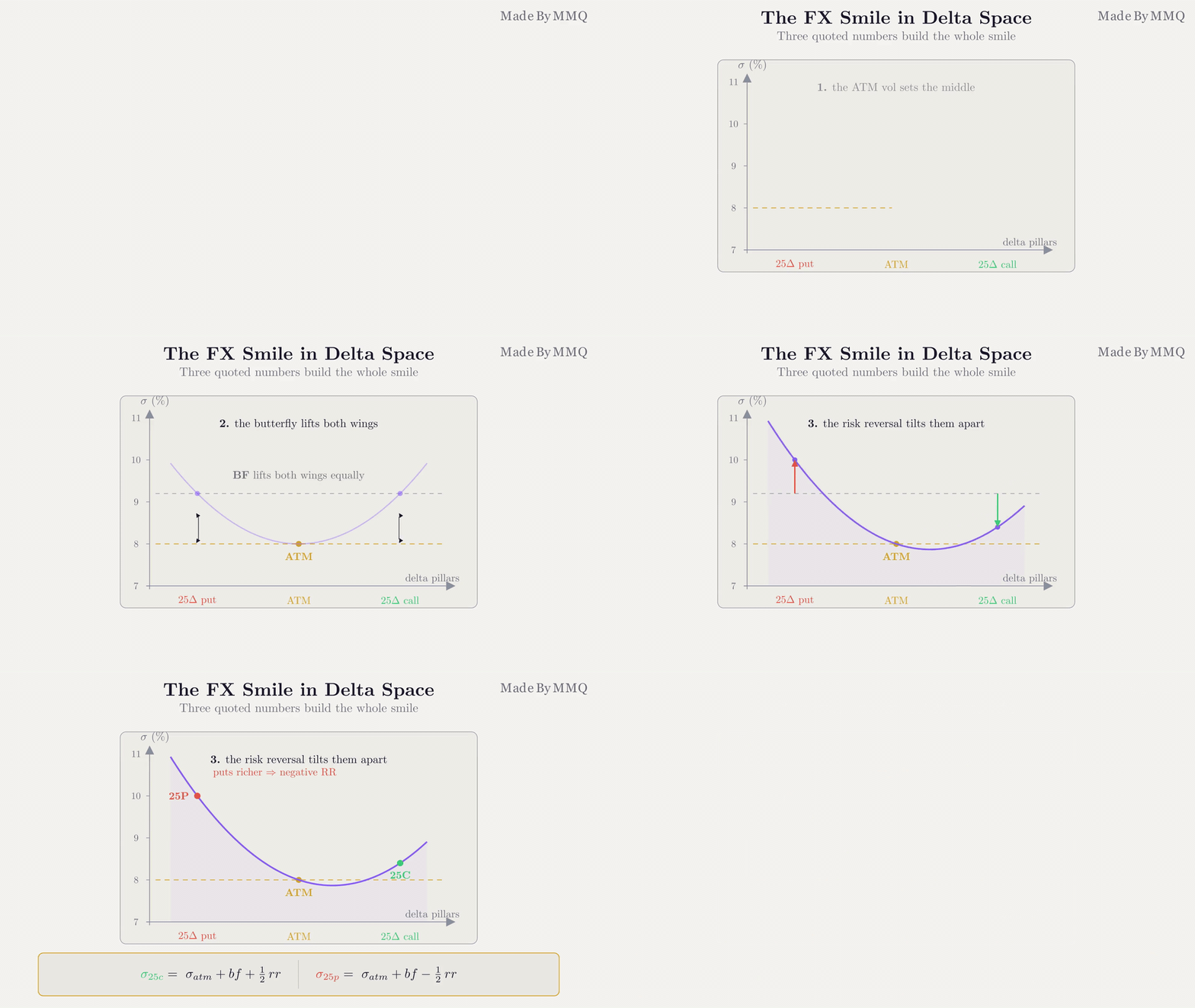
Fig. 1. The delta-space smile. The ATM vol sets the middle, the risk reversal tilts it, and the butterfly lifts the wings.
Because the input is three numbers per expiry rather than a chain, the natural way to feed the tool is a small table, one row per tenor. Here is the head of the EURUSD sample sheet shipped with the project. Volatilities are in percent, rates in decimals, and the last two columns carry the domestic and foreign interest rates that Garman-Kohlhagen needs:
| tenor | days | spot | atm | rr25 | bf25 | rr10 | bf10 | r_dom | r_for |
|---|---|---|---|---|---|---|---|---|---|
| 1W | 7 | 1.0850 | 7.50 | -0.20 | 0.15 | -0.40 | 0.50 | 0.0430 | 0.0250 |
| 1M | 30 | 1.0850 | 7.80 | -0.25 | 0.18 | -0.50 | 0.60 | 0.0430 | 0.0250 |
| 3M | 91 | 1.0850 | 8.10 | -0.30 | 0.20 | -0.60 | 0.70 | 0.0430 | 0.0250 |
The optional 10-delta columns let the sheet carry a five-point smile (10-delta put, 25-delta put, ATM, 25-delta call, 10-delta call) instead of a three-point one; set them to zero and the tool builds three pillars. One caveat on the rate columns: Garman-Kohlhagen's e^(-rT) factors assume continuously compounded rates, while a money-market deposit is quoted as simple interest on its own day-count basis. Convert with r = ln(1 + r_simple * d/b) / T before the number goes in the sheet, or the forward and every strike solved off it carry the bias. We start with the pricer.
Garman-Kohlhagen: Pricing in a Two-Rate World
The Garman-Kohlhagen model is Black-Scholes adapted to currencies. The one structural change is that the underlying, a currency, earns interest. If you hold the base currency you earn the foreign money-market rate on it, so from the perspective of the domestic currency the base leg pays a continuous yield exactly like a dividend. Black-Scholes already has a slot for a continuous yield; Garman-Kohlhagen simply fills it with the foreign rate. Everything else, the log-normal dynamics, the two discount factors, follows.
One naming trap is worth clearing before any of this reaches a spreadsheet. In FX the base currency (the one on the left, quoted in units of the other) is the foreign currency, and the quote currency is the domestic one. So for EURUSD, rd is the USD rate and rf the EUR rate; for USDJPY the same dollar rate is now rf. The sample sheets show it: the 4.30% dollar rate sits in the r_dom column of the EURUSD sheet and the r_for column of the USDJPY one. Swapping them does not throw an error, it just prices the wrong carry.
With spot S, strike K, domestic rate rd, foreign rate rf, volatility sigma and time T, the call and put are:
C = S e^(-rf T) N(d1) - K e^(-rd T) N(d2)
P = K e^(-rd T) N(-d2) - S e^(-rf T) N(-d1)

d1 = [ ln(S/K) + (rd - rf + sigma^2 / 2) T ] / ( sigma sqrt(T) )
d2 = d1 - sigma sqrt(T)
The base leg is discounted at the foreign rate, the strike leg at the domestic rate. That two-rate structure is the whole of the FX adaptation, and it is cleanest to express it once through the forward. A currency position funds at the domestic rate and earns the foreign rate, so its drift is the rate differential, and the forward is the spot carried at that differential:
//+------------------------------------------------------------------+
//| The forward FX rate. A currency position earns the foreign rate  |
//| and funds at the domestic rate, so the drift is (rd - rf) and    |
//| the forward is the spot carried at that differential. Every      |
//| Garman-Kohlhagen quantity below is cleanest expressed through    |
//| this forward, so we compute it once here.                        |
//+------------------------------------------------------------------+
double GKForward(const double S, const double rd, const double rf, const double T)
  {
   return(S * MathExp((rd - rf) * T));
  }
The pricer itself is the textbook formula above, guarded so degenerate inputs never reach the d1 term. Those guards repay a moment's thought, because the obvious version is wrong. At or past expiry the value is spot intrinsic. But with time still to run and a zero volatility the payoff is deterministic on the forward, not the spot, so the value is that intrinsic discounted at the domestic rate: e^(-rd T) max(F - K, 0) for a call, which is also what the formula converges to as sigma falls to zero. On the shipped sample that is worth about 16 pips, since a 30-day EURUSD call struck at spot is worth 0.00160 at zero vol where a spot-intrinsic reading calls it worthless. The standard normal CDF is the same Abramowitz and Stegun approximation used in the surface tool, cheap enough for the solver's inner loop; we reuse it as NormCDF and measure its error later.
//+------------------------------------------------------------------+
//| Garman-Kohlhagen price of a European FX option. This is Black-   |
//| Scholes with the foreign interest rate playing the role of a     |
//| continuous dividend yield on the base currency: the base leg is  |
//| discounted at rf, the strike leg at the domestic rate rd. At or  |
//| past expiry value is spot intrinsic; with time left but zero vol |
//| the payoff is deterministic on the FORWARD, so it is that        |
//| intrinsic discounted at rd, which is also the sigma -> 0 limit   |
//| of the formula below.                                            |
//+------------------------------------------------------------------+
double GKPrice(const ENUM_OPT_RIGHT right, const double S, const double K,
               const double rd, const double rf, const double sigma, const double T)
  {
   if(S <= 0.0 || K <= 0.0)
      return(0.0);
   if(T <= 0.0)
      return((right == OPT_CALL) ? MathMax(S - K, 0.0) : MathMax(K - S, 0.0));
   if(sigma <= 0.0)
     {
      //--- zero vol, time left: discounted deterministic payoff on the forward
      double Fz = GKForward(S, rd, rf, T);
      double vz = (right == OPT_CALL) ? MathMax(Fz - K, 0.0) : MathMax(K - Fz, 0.0);
      return(MathExp(-rd * T) * vz);
     }
   double sqrtT = MathSqrt(T);
   double d1    = (MathLog(S / K) + (rd - rf + 0.5 * sigma * sigma) * T) / (sigma * sqrtT);
   double d2    = d1 - sigma * sqrtT;
   double dfDom = MathExp(-rd * T);
   double dfFor = MathExp(-rf * T);
   if(right == OPT_CALL)
      return(S * dfFor * NormCDF(d1) - K * dfDom * NormCDF(d2));
   else
      return(K * dfDom * NormCDF(-d2) - S * dfFor * NormCDF(-d1));
  }
A cheap but reassuring check on this function is put-call parity, which for FX reads C - P = S e^(-rf T) - K e^(-rd T). It holds to machine precision, because both legs are built from the same two discount factors. Be clear about what that buys: it tests the pricer's internal consistency and nothing else, and would close just as cleanly on a wrong volatility, rate or delta convention.
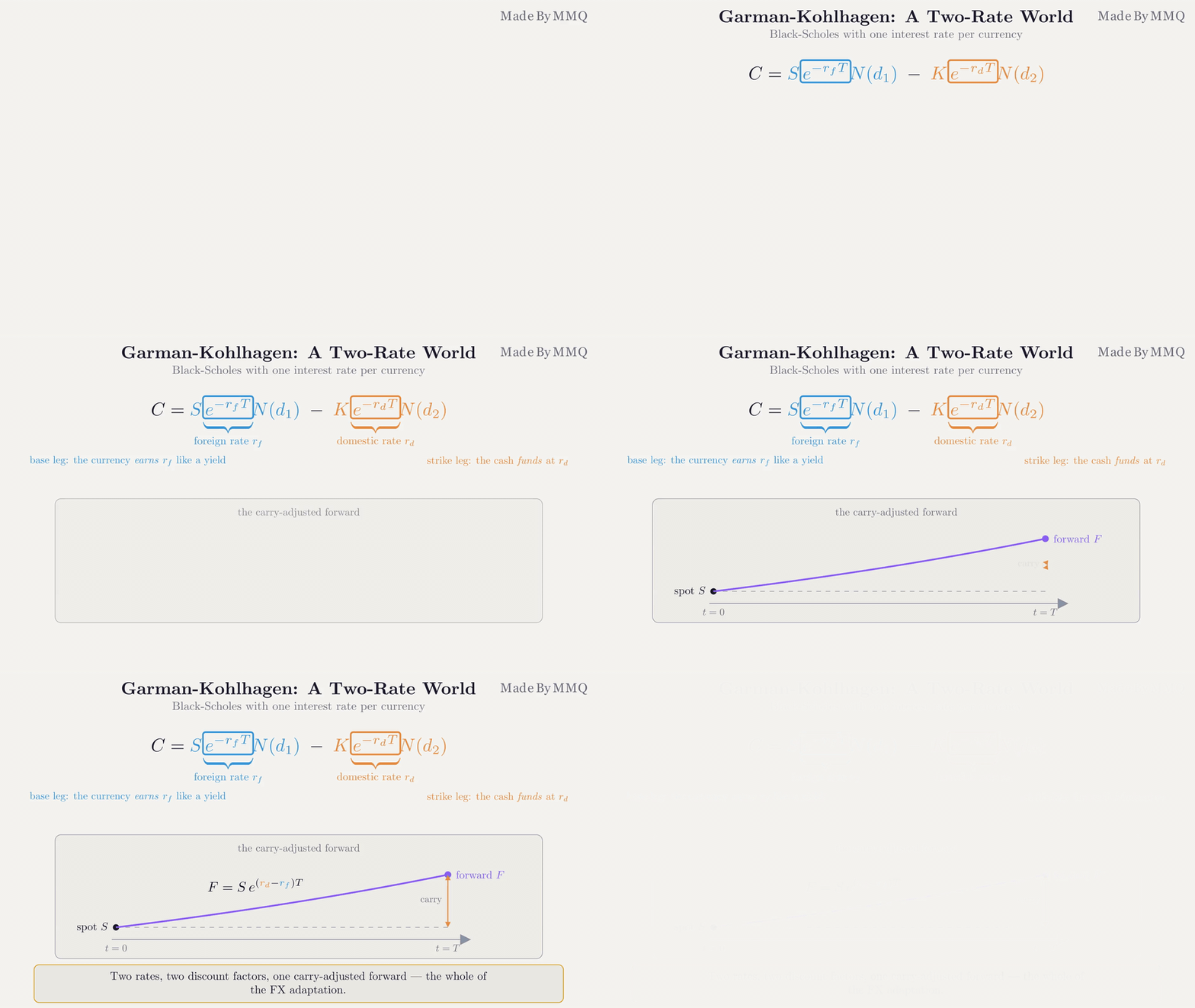
Fig. 2. The two-rate world: the base leg discounts at the foreign rate, the strike leg at the domestic rate, and the forward carries the spot at their difference.
The Greeks, and why FX has two rhos
The header carries the full set of Greeks: gamma, vega and theta follow the same two-rate pattern as the price, with the base-currency terms discounted at the foreign rate, and theta carries both carry terms an equity option lacks. The most visibly FX-specific Greek is rho: an equity option has one interest-rate sensitivity, an FX option has two, one per rate, moving in opposite directions. The domestic rho acts through the discounted strike leg, the foreign rho through the base leg:
//+------------------------------------------------------------------+
//| Rho to the domestic rate: sensitivity of value to a 1.00 change  |
//| in rd, acting through the discounted strike leg. FX has two of   |
//| these, one per rate, which is the structural break from the      |
//| single-rho equity Greeks.                                        |
//+------------------------------------------------------------------+
double GKRhoDom(const ENUM_OPT_RIGHT right, const double S, const double K, const double rd,
                const double rf, const double sigma, const double T)
  {
   if(T <= 0.0 || sigma <= 0.0 || S <= 0.0 || K <= 0.0)
      return(0.0);
   double sqrtT = MathSqrt(T);
   double d1    = (MathLog(S / K) + (rd - rf + 0.5 * sigma * sigma) * T) / (sigma * sqrtT);
   double d2    = d1 - sigma * sqrtT;
   double dfDom = MathExp(-rd * T);
   if(right == OPT_CALL)
      return(K * T * dfDom * NormCDF(d2));
   else
      return(-K * T * dfDom * NormCDF(-d2));
  }
The foreign rho is its mirror through the base leg, returning -S T e^(-rf T) N(d1) for a call. Both rhos appear in the indicator's header later, a reminder that an FX option's value responds to two yield curves, not one.
The Delta Is a Convention
This is the section that separates a correct FX smile from a plausible-looking wrong one. In the equity world delta is unambiguous, the partial derivative of value with respect to spot. In FX four different quantities all get called "the delta", and a 25-delta is only a 25-delta once you have said which.
The four arise from two independent binary choices: the delta can be measured on the spot or the forward, and it can be premium-adjusted or not. The unadjusted spot delta is the raw hedge ratio, e^(-rf T) N(d1); dropping the discount factor gives the forward delta. The premium-adjusted variants exist because when the premium is paid in the base currency it carries FX risk of its own, and the hedge must net it out, which turns the N(d1) term into a (K/F) N(d2) term:
spot delta, unadjusted: phi e^(-rf T) N(phi d1)
forward delta, unadjusted: phi N(phi d1)
spot delta, premium-adjusted: phi e^(-rf T) (K/F) N(phi d2)
forward delta, premium-adjusted: phi (K/F) N(phi d2)
Here phi is +1 for a call and -1 for a put, so one expression covers both rights, with ENUM_OPT_RIGHT carrying the choice. All four conventions live in one function, selected by an enum, so the rest of the code asks for "the delta under this convention" and never has to know the algebra:
//+------------------------------------------------------------------+
//| Delta under a chosen FX convention. The unadjusted spot delta,   |
//| e^(-rf T) N(d1), is the raw hedge ratio in base-currency units.  |
//| Dropping the e^(-rf T) discount gives the forward delta. The     |
//| premium-adjusted variants subtract the option's own base-        |
//| currency premium from the hedge, which turns the N(d1) term into |
//| a (K/F) N(d2) term. Puts carry the mirror sign throughout.       |
//+------------------------------------------------------------------+
double GKDelta(const ENUM_OPT_RIGHT right, const ENUM_GK_DELTA conv, const double S,
               const double K, const double rd, const double rf, const double sigma, const double T)
  {
   if(T <= 0.0 || sigma <= 0.0 || S <= 0.0 || K <= 0.0)
      return(0.0);
   double sqrtT = MathSqrt(T);
   double F     = GKForward(S, rd, rf, T);
   double d1    = (MathLog(S / K) + (rd - rf + 0.5 * sigma * sigma) * T) / (sigma * sqrtT);
   double d2    = d1 - sigma * sqrtT;
   double phi   = (right == OPT_CALL) ? 1.0 : -1.0;
   double dfFor = MathExp(-rf * T);

   switch(conv)
     {
      case GK_DELTA_SPOT:
         return(phi * dfFor * NormCDF(phi * d1));
      case GK_DELTA_FORWARD:
         return(phi * NormCDF(phi * d1));
      case GK_DELTA_SPOT_PA:
         return(phi * dfFor * (K / F) * NormCDF(phi * d2));
      case GK_DELTA_FORWARD_PA:
         return(phi * (K / F) * NormCDF(phi * d2));
     }
   return(0.0);
  }
Which pair uses which is not something you pick to taste. The rule behind the table follows from the paragraph above: on the dollar pairs the premium is conventionally paid in US dollars. When the dollar is the quote currency, as in EURUSD, the premium lands in the domestic currency and carries no FX risk, so the delta is unadjusted. When it is the base currency, as in USDJPY, the premium is itself an exposure to the underlying and has to be netted out. Crosses follow the same logic through their own premium currency, and at long tenors many sources move to forward delta because the discount factor stops being a rounding detail:
| Pair | Delta measured on | Premium-adjusted? |
|---|---|---|
| EURUSD, GBPUSD, AUDUSD, NZDUSD | spot | No (unadjusted) |
| USDJPY, USDCHF, USDCAD | spot | Yes |
| EURJPY and most crosses | spot | Yes |
| Long tenors, commonly from 1Y to 2Y outward | forward | as above |
Read that table as the common default rather than a rule. The premium currency is a term of the contract, not a property of the pair, and it, the delta convention and the tenor at which forward delta takes over all travel with the quote source. Take them from whoever supplies your volatilities, which is why the tool exposes them as inputs instead of hard-coding a lookup by symbol.
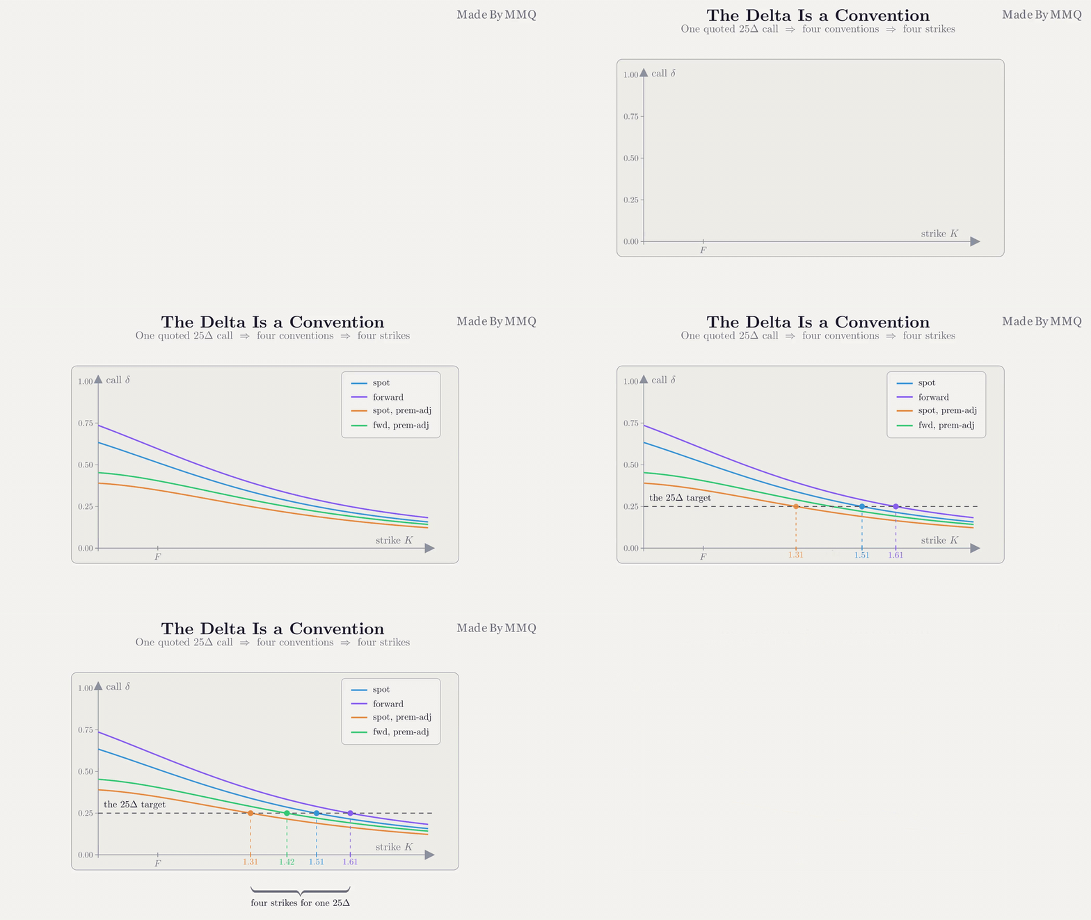
Fig. 3. One quoted 25-delta, four conventions, four different strikes on the same smile.
The at-the-money strike is convention-dependent for the same reason. "At the money" in FX usually means the delta-neutral straddle, the strike where a call and a put share the same absolute delta. Solving that condition puts the ATM strike half a variance above the forward under an unadjusted delta and half below it under a premium-adjusted one, because the premium term shifts the delta that has to net to zero. The alternative convention is simply the forward. Both are handled in one place:
//+------------------------------------------------------------------+
//| The ATM strike for a given ATM and delta convention. The delta-  |
//| neutral straddle sits half a variance above the forward under an |
//| unadjusted delta, and half a variance below it under a premium-  |
//| adjusted delta, because the premium term shifts the delta that   |
//| has to net to zero. The forward convention is just F. Getting    |
//| this strike wrong offsets the entire smile by its ATM anchor.    |
//+------------------------------------------------------------------+
double GKATMStrike(const ENUM_GK_ATM atmConv, const ENUM_GK_DELTA deltaConv,
                   const double F, const double sigma, const double T)
  {
   if(atmConv == GK_ATM_FORWARD)
      return(F);
//--- delta-neutral straddle: sign of the half-variance shift depends
//--- on whether the delta is premium-adjusted
   bool pa = (deltaConv == GK_DELTA_SPOT_PA || deltaConv == GK_DELTA_FORWARD_PA);
   double half = 0.5 * sigma * sigma * T;
   return(pa ? F * MathExp(-half) : F * MathExp(half));
  }
The ATM convention is a second per-pair choice, exposed separately as InpAtmConv, and it is not implied by the delta convention. The liquid G10 pairs quote the delta-neutral straddle, the default here; some emerging-market and long-dated quotes are published against the at-the-money forward instead. It travels with the quote, so take it from whoever supplies the vols: the two settings differ by exactly the half-variance shift above.
How much does the convention actually move a strike?
The honest answer depends heavily on the tenor. Both the premium adjustment and the ATM shift are governed by the variance sigma^2 T, so the effect is negligible at a week and large at a year. The table below runs the shipped sheets through the reconstruction twice, once on each spot convention, and reports the gap:
| Sheet row | 25d call K, unadjusted | 25d call K, premium-adjusted | Gap, pips | ATM strike gap, pips |
|---|---|---|---|---|
| EURUSD 1M | 1.10348 | 1.10321 | 2.6 | 5.5 |
| EURUSD 1Y | 1.17259 | 1.16844 | 41.5 | 79.8 |
| USDJPY 1M | 152.147 | 152.099 | 4.8 | 11.1 |
| USDJPY 1Y | 153.317 | 152.665 | 65.2 | 149.6 |
At one month the convention is worth a few pips, which you will not see on a chart. At one year it is worth 40 to 65 pips on the wing and, on USDJPY, a full 1.5 yen on the ATM anchor itself, which is the difference between a ladder a desk recognises and one it does not. The convention is not a detail you can defer, but its cost grows with the tenor. Fig. 3 above is drawn at a deliberately long, high-volatility setting so the four curves separate visibly; on a one-week sheet all four would sit nearly on top of one another.
With the delta pinned down as a convention rather than a single formula, we can finally do the reconstruction: turn the three quoted numbers into the strikes and vols of an actual smile.
From Three Quotes to a Smile: Reconstruction
Reconstruction is the heart of the tool. The input is a row of quotes, ATM plus the risk reversals and butterflies; the output is a set of points, each a strike with the volatility that lives on it. Two data structures carry that output: a point is a strike, its vol and the delta actually realised there, which lets a caller confirm a "25-delta" pillar really sits at 0.25; a tenor bundles the raw quotes, the market data and, once built, the reconstructed points:
//+------------------------------------------------------------------+
//| One reconstructed point on a tenor's smile: the strike a quoted  |
//| delta pillar maps to, the volatility that lives there, and the   |
//| realised delta at that strike (which pins the pillar it came     |
//| from). Ordered left to right by strike, these five points are    |
//| the smile the FX market only ever quotes in delta space.         |
//+------------------------------------------------------------------+
struct SmilePoint
  {
   string            label;    // "10P","25P","ATM","25C","10C"
   double            strike;   // reconstructed strike
   double            vol;      // volatility at this strike (decimal)
   double            delta;    // realised delta at the strike (signed)
  };
The reconstruction runs in two steps. First it turns the quoted structures into the volatilities at each pillar, using the simplified smile-strangle reading: the risk reversal splits the wings around the butterfly-lifted average, so the 25-delta call vol is ATM plus butterfly plus half the risk reversal, and the put vol the same with half subtracted. Second, it solves each pillar's delta back to the strike it lives on, at that pillar's own vol.
The strike solve is the one genuinely delicate numeric step, because of the non-monotonicity flagged earlier. Holding the vol fixed, we want the strike whose delta equals the target. For an unadjusted delta that strike is unique; for a premium-adjusted call it is not, since the delta rises then falls, so there are two and the convention takes the larger, out-of-the-money one. Scanning from high to low and bracketing the first sign change returns exactly that root, and the unique root otherwise, so one routine handles all four conventions:
//+------------------------------------------------------------------+
//| Invert a target delta to its strike, holding sigma fixed. Used   |
//| to turn each quoted delta pillar (10d, 25d) into the strike the  |
//| smile actually lives on. The unadjusted delta is monotonic in    |
//| the strike, but the premium-adjusted call delta is not: it rises |
//| then falls, so a 25-delta call has two strikes and the market    |
//| convention takes the larger (out-of-the-money) one. Scanning the |
//| strike axis from high to low and bracketing the first sign       |
//| change returns exactly that root, and the unique root otherwise. |
//|                                                                  |
//| targetAbs is the delta magnitude (e.g. 0.25); the sign is taken  |
//| from the right. Returns a negative sentinel if no strike matches.|
//+------------------------------------------------------------------+
double GKStrikeFromDelta(const ENUM_OPT_RIGHT right, const ENUM_GK_DELTA conv, const double targetAbs,
                         const double S, const double rd, const double rf, const double sigma, const double T)
  {
   if(T <= 0.0 || sigma <= 0.0 || S <= 0.0 || targetAbs <= 0.0)
      return(-1.0);
   double target = (right == OPT_CALL) ? targetAbs : -targetAbs;
   double F      = GKForward(S, rd, rf, T);

//--- scan log-strike space around the forward, high to low, for a
//--- sign change of (delta - target); K in [F*e^-3, F*e^+3] is ample
   int    steps = 400;
   double kHi   = F * MathExp(3.0);
   double kLo   = F * MathExp(-3.0);
   double logHi = MathLog(kHi), logLo = MathLog(kLo);
   double prevK = kHi;
   double prevF = GKDelta(right, conv, S, prevK, rd, rf, sigma, T) - target;

   for(int i = 1; i <= steps; i++)
     {
      double frac = (double)i / steps;
      double curK = MathExp(logHi + (logLo - logHi) * frac);
      double curF = GKDelta(right, conv, S, curK, rd, rf, sigma, T) - target;
      if(prevF == 0.0)
         return(prevK);
      if(prevF * curF < 0.0)
        {
         //--- bracket found: bisect [curK, prevK] to a tight strike
         double a = curK, b = prevK, fa = curF;
         for(int j = 0; j < 100; j++)
           {
            double m  = 0.5 * (a + b);
            double fm = GKDelta(right, conv, S, m, rd, rf, sigma, T) - target;
            if(MathAbs(fm) < 1e-12 || (b - a) < 1e-10)
               return(m);
            if(fa * fm < 0.0)
               b = m;
            else
              {
               a  = m;
               fa = fm;
              }
           }
         return(0.5 * (a + b));
        }
      prevK = curK;
      prevF = curF;
     }
   return(-1.0);
  }
The scan window deserves a number rather than an assurance. A pillar sits at ln(K/F) = -d1 sigma sqrt(T) + 0.5 sigma^2 T, and the widest we ask for is the 10-delta, where |d1| is about 1.28. Setting that equal to the window's half-width of 3 gives 0.5 x^2 + 1.28 x = 3 with x = sigma sqrt(T), so the bracket is exhausted only near sigma sqrt(T) = 1.48: about 148% volatility at one year, or 66% at five, against the sheets' 7.5% to 10.2%. That is the figure to re-check before pointing the tool at a crisis-period emerging-market pair, and if it is ever breached the scan finds no sign change and returns a negative sentinel rather than a wrong strike.
With the vols and the strike solver in hand, building one tenor is a short, readable sequence. It derives the pillar vols, then places each pillar by solving its delta back to a strike, putting the put pillars in first so the finished points stay in ascending strike order. Every pillar also records the delta realised at its solved strike, the built-in check: if a "25P" pillar comes back at anything other than -0.25, the solve is wrong. Should a solve fail, AddPoint drops that pillar rather than pushing a bad strike into the smile.
//+------------------------------------------------------------------+
//| Reconstruct one tenor's smile. Derive the pillar vols from the   |
//| ATM/RR/BF quotes, solve each pillar delta back to a strike using |
//| that pillar's own vol, and record the realised delta. The put    |
//| pillars are solved to negative deltas, the calls to positive; a  |
//| correct convention returns strikes that stay in ascending order  |
//| 10P < 25P < ATM < 25C < 10C.                                     |
//+------------------------------------------------------------------+
void CGKSmile::BuildTenor(SmileTenor &t)
  {
   t.T = t.days / 365.0;
   t.F = GKForward(t.spot, t.rd, t.rf, t.T);
   ArrayResize(t.pts, 0);

//--- pillar vols from the delta-space quotes (simplified strangle)
   double s25c = t.atm + t.bf25 + 0.5 * t.rr25;
   double s25p = t.atm + t.bf25 - 0.5 * t.rr25;

//--- pillar strikes (put pillars first so points stay ascending)
   if(t.has10)
     {
      double s10c = t.atm + t.bf10 + 0.5 * t.rr10;
      double s10p = t.atm + t.bf10 - 0.5 * t.rr10;
      double k10p = GKStrikeFromDelta(OPT_PUT, m_dconv, 0.10, t.spot, t.rd, t.rf, s10p, t.T);
      AddPoint(t, "10P", k10p, s10p, GKDelta(OPT_PUT, m_dconv, t.spot, k10p, t.rd, t.rf, s10p, t.T));
     }
   double k25p = GKStrikeFromDelta(OPT_PUT, m_dconv, 0.25, t.spot, t.rd, t.rf, s25p, t.T);
   AddPoint(t, "25P", k25p, s25p, GKDelta(OPT_PUT, m_dconv, t.spot, k25p, t.rd, t.rf, s25p, t.T));

   double kAtm = GKATMStrike(m_aconv, m_dconv, t.F, t.atm, t.T);
   AddPoint(t, "ATM", kAtm, t.atm, GKDelta(OPT_CALL, m_dconv, t.spot, kAtm, t.rd, t.rf, t.atm, t.T));

   double k25c = GKStrikeFromDelta(OPT_CALL, m_dconv, 0.25, t.spot, t.rd, t.rf, s25c, t.T);
   AddPoint(t, "25C", k25c, s25c, GKDelta(OPT_CALL, m_dconv, t.spot, k25c, t.rd, t.rf, s25c, t.T));

   if(t.has10)
     {
      double s10c = t.atm + t.bf10 + 0.5 * t.rr10;
      double k10c = GKStrikeFromDelta(OPT_CALL, m_dconv, 0.10, t.spot, t.rd, t.rf, s10c, t.T);
      AddPoint(t, "10C", k10c, s10c, GKDelta(OPT_CALL, m_dconv, t.spot, k10c, t.rd, t.rf, s10c, t.T));
     }
  }
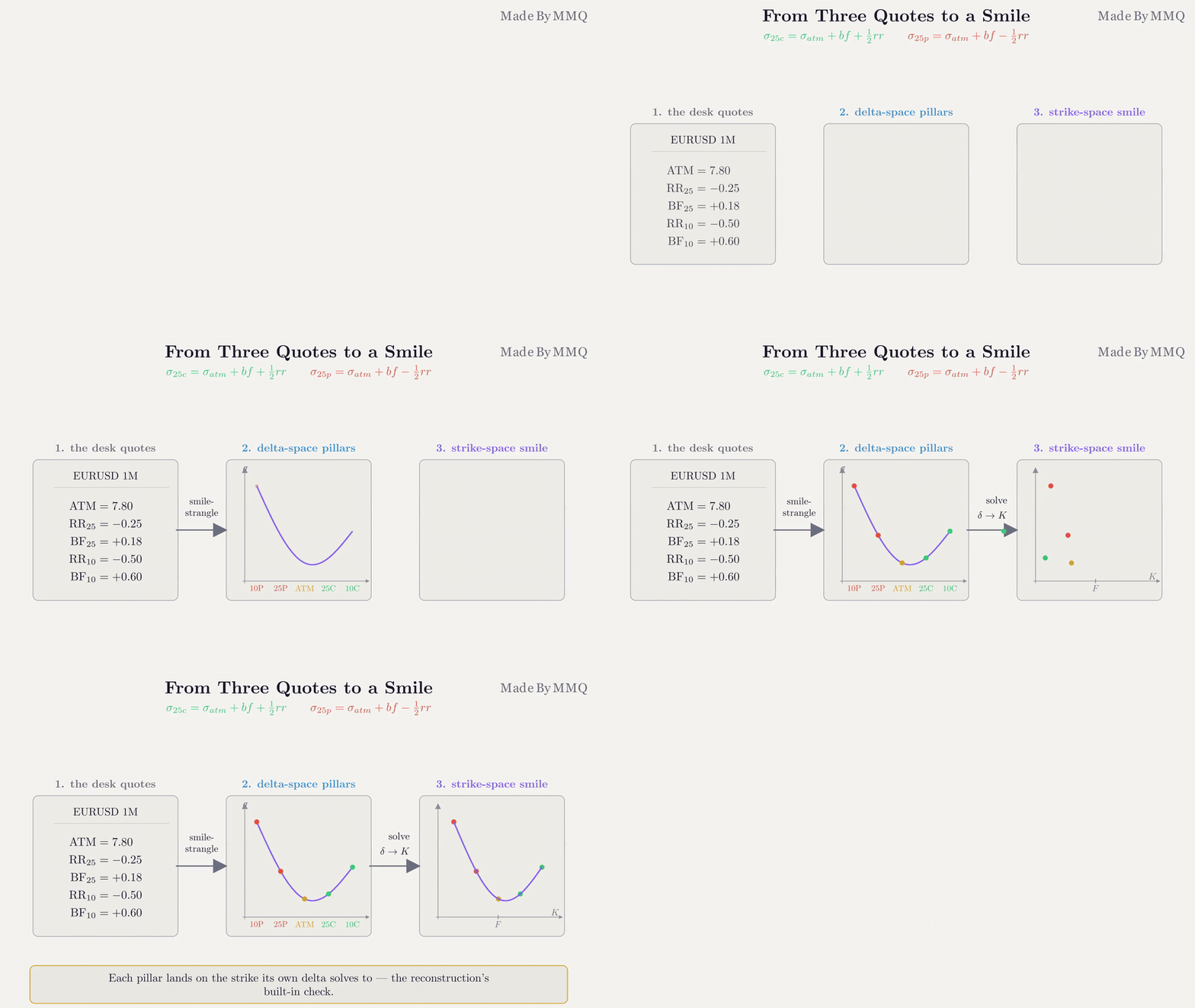
Fig. 4. Reconstruction turns three quoted numbers into five strike-space pillars, each solved back to the strike its delta lives on.
The public Build method loops this over every tenor and takes ownership of the result, exposing it through accessors for tenor labels, forwards and per-pillar strikes, vols and deltas. The drawing code reads them without caring how any of it was computed.
Checking the reconstruction against an independent implementation
The realised-delta field turns the reconstruction into something we can test rather than eyeball. The check below is a second implementation of the same maths in Python, written from the formulas rather than translated from the header, and differing in one deliberate way: it takes its normal CDF from math.erfc, exact to double precision, where the header uses Abramowitz and Stegun. That establishes the formulas are right and says nothing yet about the MQL5 that ships, a gap we close immediately afterwards. It is reproduced in full rather than attached:
#--- Independent Python reference for the MQL5 reconstruction. math.erfc is
#--- exact to double precision, so agreement with the header's Abramowitz &
#--- Stegun NormCDF also bounds the error of that approximation.
from math import exp, log, sqrt, erfc

def N(x):
    return 0.5 * erfc(-x / sqrt(2.0))

def forward(S, rd, rf, T):
    return S * exp((rd - rf) * T)

def delta(right, conv, S, K, rd, rf, sg, T):
    F  = forward(S, rd, rf, T)
    d1 = (log(S / K) + (rd - rf + 0.5 * sg * sg) * T) / (sg * sqrt(T))
    d2 = d1 - sg * sqrt(T)
    ph = 1.0 if right == "C" else -1.0
    df = exp(-rf * T)
    if conv == "spot":    return ph * df * N(ph * d1)
    if conv == "fwd":     return ph * N(ph * d1)
    if conv == "spot_pa": return ph * df * (K / F) * N(ph * d2)
    return ph * (K / F) * N(ph * d2)

def strike_from_delta(right, conv, tgt, S, rd, rf, sg, T):
    #--- the same scan high-to-low then bisect as GKStrikeFromDelta
    tar = tgt if right == "C" else -tgt
    hi  = log(forward(S, rd, rf, T)) + 3.0
    lo  = hi - 6.0
    pk  = exp(hi); pf = delta(right, conv, S, pk, rd, rf, sg, T) - tar
    for i in range(1, 401):
        ck = exp(hi + (lo - hi) * i / 400.0)
        cf = delta(right, conv, S, ck, rd, rf, sg, T) - tar
        if pf * cf < 0.0:
            a, b, fa = ck, pk, cf
            for _ in range(100):
                m  = 0.5 * (a + b)
                fm = delta(right, conv, S, m, rd, rf, sg, T) - tar
                if abs(fm) < 1e-12 or (b - a) < 1e-10: return m
                if fa * fm < 0.0: b = m
                else:             a, fa = m, fm
            return 0.5 * (a + b)
        pk, pf = ck, cf
    return -1.0

def build(conv, S, rd, rf, days, atm, rr25, bf25, rr10, bf10):
    T, F = days / 365.0, forward(S, rd, rf, days / 365.0)
    half = 0.5 * atm * atm * T
    kAtm = F * exp(-half) if conv.endswith("_pa") else F * exp(half)
    v = {"10P": atm + bf10 - 0.5 * rr10, "25P": atm + bf25 - 0.5 * rr25, "ATM": atm,
         "25C": atm + bf25 + 0.5 * rr25, "10C": atm + bf10 + 0.5 * rr10}
    out = []
    for lab, tgt, r in [("10P", 0.10, "P"), ("25P", 0.25, "P"), ("ATM", None, "C"),
                        ("25C", 0.25, "C"), ("10C", 0.10, "C")]:
        K = kAtm if tgt is None else strike_from_delta(r, conv, tgt, S, rd, rf, v[lab], T)
        out.append((lab, K, v[lab], delta(r, conv, S, K, rd, rf, v[lab], T), tgt))
    return F, out
The pieces above mirror the header one for one: delta carries the same four conventions, and strike_from_delta repeats the scan high-to-low then bisect that handles the non-monotonic premium-adjusted call. The driver then rebuilds the EURUSD 1M row straight off the shipped sheet, sweeps every tenor of both sheets under all four conventions, and closes with put-call parity:
#--- EURUSD 1M, read straight off the shipped sheet
F, pts = build("spot", 1.0850, 0.0430, 0.0250, 30, 0.0780, -0.0025, 0.0018, -0.0050, 0.0060)
print("EURUSD 1M   spot 1.08500   forward %.5f" % F)
for lab, K, vol, d, tgt in pts:
    print("  %-3s  K = %8.5f   vol = %6.3f%%   realised delta = %+9.6f" % (lab, K, vol * 100.0, d))
print("  ascending 10P < 25P < ATM < 25C < 10C :",
      all(pts[i][1] < pts[i + 1][1] for i in range(4)))

#--- worst pillar error over both sheets, every tenor, all four conventions
EUR = [(7, .0750, -.0020, .0015, -.0040, .0050), (30, .0780, -.0025, .0018, -.0050, .0060),
       (91, .0810, -.0030, .0020, -.0060, .0070), (182, .0830, -.0035, .0022, -.0070, .0080),
       (365, .0850, -.0040, .0025, -.0080, .0090)]
JPY = [(7, .0900, -.0120, .0020, -.0230, .0070), (30, .0950, -.0150, .0025, -.0280, .0085),
       (91, .0980, -.0180, .0030, -.0330, .0100), (182, .1000, -.0210, .0033, -.0380, .0110),
       (365, .1020, -.0250, .0035, -.0430, .0125)]
worst = 0.0
for S, rd, rf, rows in [(1.0850, .0430, .0250, EUR), (150.0, .0010, .0430, JPY)]:
    for conv in ["spot", "fwd", "spot_pa", "fwd_pa"]:
        for row in rows:
            for lab, K, vol, d, tgt in build(conv, S, rd, rf, *row)[1]:
                if tgt is not None:
                    worst = max(worst, abs(abs(d) - tgt))
print("worst |realised delta - target|, 2 sheets x 5 tenors x 4 conventions: %.2e" % worst)

#--- put-call parity: C - P = S e^(-rf T) - K e^(-rd T)
S, K, rd, rf, sg, T = 1.0850, 1.0900, 0.0430, 0.0250, 0.0780, 30 / 365.0
d1 = (log(S / K) + (rd - rf + 0.5 * sg * sg) * T) / (sg * sqrt(T))
d2 = d1 - sg * sqrt(T)
C  = S * exp(-rf * T) * N(d1) - K * exp(-rd * T) * N(d2)
P  = K * exp(-rd * T) * N(-d2) - S * exp(-rf * T) * N(-d1)
print("put-call parity residual: %.2e" % abs((C - P) - (S * exp(-rf * T) - K * exp(-rd * T))))
Running it prints:
EURUSD 1M   spot 1.08500   forward 1.08661
  10P  K =  1.05297   vol =  8.650%   realised delta = -0.100000
  25P  K =  1.07004   vol =  8.105%   realised delta = -0.250000
  ATM  K =  1.08688   vol =  7.800%   realised delta = +0.498974
  25C  K =  1.10348   vol =  7.855%   realised delta = +0.250000
  10C  K =  1.11991   vol =  8.150%   realised delta = +0.100000
  ascending 10P < 25P < ATM < 25C < 10C : True
worst |realised delta - target|, 2 sheets x 5 tenors x 4 conventions: 7.80e-10
put-call parity residual: 0.00e+00
Three things fall out of that. The pillars land in ascending strike order, so the smile is a function of the strike rather than a curve that doubles back. Every solved pillar returns the delta it was asked for to within 7.8e-10, across two pairs, five tenors and all four conventions, which is the bisection's own strike tolerance rather than any modelling error, and put-call parity closes at a residual of zero on this reference. The ATM pillar sitting at +0.498974 rather than a round 0.500 is not an error either: it is the e^(-rf T) discount on the unadjusted spot delta, exactly what a delta-neutral straddle should show under this convention.
Be careful what that delta figure proves. The strike is found by solving the delta function and the realised delta is measured with the same function, so it is a statement about the solver, not about the finance: it confirms the bisection converges, that the non-monotonic premium-adjusted branch picks the out-of-the-money root, and that the pillars stay ordered. It cannot confirm the delta convention is the one your counterparty uses, and neither can parity. Those are inputs you have to get right from the quote source.
Comparing the header against the reference, not just describing it
Everything above runs in Python, which is a reference agreeing with itself and not yet evidence about the code you will attach to a chart. So the last step puts the two side by side. An MQL5 script loads both shipped sheets through the real CSV provider, reconstructs them under all four conventions, and writes every strike, vol and realised delta with StringFormat's %.17g, which round-trips a double exactly; Python reads the same sheets, rebuilds them from the listing above, and diffs the two sets on a sheet, convention, tenor and pillar key. The same run records NormCDF on a fine grid, so the approximation is measured against math.erfc rather than inferred:
pillars compared (2 sheets x 5 tenors x 4 conventions) : 200
Python on math.erfc vs MQL5 on Abramowitz & Stegun
  worst relative strike difference                     : 5.075e-08
  worst relative vol difference                        : 0.000e+00
  worst absolute realised-delta difference             : 1.163e-09
Python rebuilt on the SAME Abramowitz & Stegun CDF
  worst relative strike difference                     : 0.000e+00
  worst absolute realised-delta difference             : 0.000e+00
NormCDF over x in [-8,8], step 1e-4, 160001 points
  worst absolute error vs math.erfc                    : 7.452e-08  at x = -0.7173
put-call parity residual, MQL5 GKPrice                 : 1.110e-16
zero-vol guard vs closed form and the sigma -> 0 limit : 2.220e-16
GKPrice(S = -1), GKPrice(K = -1)                       : 0, 0
The middle block settles it. Swap the Python reference's exact CDF for the header's own approximation and all 200 pillars match bit for bit, so the two are the same computation and the whole 5.1e-8 residual above is the CDF and nothing else. The pillar vols match exactly in both runs, as they should, being plain arithmetic on the quotes. That also puts a number on the approximation: worst by 7.45e-8 at x = -0.7173, within a hair of the published 7.5e-8 bound for Abramowitz and Stegun 7.1.26, and worst in the body rather than the tails. The pricer's guards check out too, the zero-vol branch agreeing with the closed form and the sigma-to-zero limit to one unit in the last place.
What this build does not model
Those checks bound the arithmetic. They say nothing about the modelling choices underneath it, which are worth naming rather than leaving to be discovered:
- One flat rate pair per tenor, not a bootstrapped curve. Real pricing builds the forward from the tenor's own curve points, and the gap grows with maturity and with the steepness of the two curves.
- Calendar days over 365 throughout. ACT/365 is the usual FX volatility clock, so that part is standard, but the same T is reused for the discount factors, where the rate's own day-count basis applies. Settlement lags, the spot date and the expiry cut are not modelled.
- No arbitrage check. Five pillars joined by straight lines can give a call-price curve that is not convex in the strike, and nothing stops neighbouring tenors crossing in total variance.
- The simplified butterfly, as the callout above sets out. A market-strangle quote needs the extra calibration step before the pillar vols are the market's own.
Two Ways to Feed It: CSV and Native
The reconstruction does not care where its quotes come from; it only needs a SmileTenor with the ATM, risk reversal and butterfly filled in. That is the seam that lets us ship two interchangeable providers. The CSV provider reads the delta-space vol sheet shown earlier and works on any account. The native provider reads the broker's own MetaTrader 5 option symbols, and has to do something more interesting, because a listed chain speaks strike space, not delta space.
The CSV provider is the straightforward one. It opens the sheet, skips the header, and turns each row into a raw tenor, converting the percent vols to decimals as it reads and flagging whether the 10-delta wings were supplied. The one guard worth having is against StringToDouble, which returns zero for anything it cannot parse, so a garbled row would otherwise load as a tidy set of zeros and reconstruct into a plausible-looking smile. Days, spot and ATM cannot legitimately be zero, so a row failing that is named in the log and dropped:
//+------------------------------------------------------------------+
//| Parse the vol sheet into raw tenors. Skips the header line and   |
//| any blank line, converts the percent vols to decimals, and       |
//| flags whether the 10-delta wings were supplied. StringToDouble   |
//| returns 0 for anything it cannot parse, so a garbled or shifted  |
//| row would load silently as zeros; days, spot and atm cannot      |
//| legitimately be zero, and a row failing that is reported and     |
//| dropped rather than reconstructed into nonsense.                 |
//+------------------------------------------------------------------+
bool CGKProviderCSV::Load(const string filename, SmileTenor &out[])
  {
   int h = FileOpen(filename, FILE_READ | FILE_CSV | FILE_ANSI, ',');
   if(h == INVALID_HANDLE)
     {
      PrintFormat("CGKProviderCSV: cannot open %s (err %d)", filename, GetLastError());
      return(false);
     }
   ArrayResize(out, 0);
   bool header = true;
   while(!FileIsEnding(h))
     {
      string sTenor = FileReadString(h);
      if(FileIsLineEnding(h) && StringLen(sTenor) == 0)
         continue;
      string sDays = FileReadString(h);
      string sSpot = FileReadString(h);
      string sAtm  = FileReadString(h);
      string sRr25 = FileReadString(h);
      string sBf25 = FileReadString(h);
      string sRr10 = FileReadString(h);
      string sBf10 = FileReadString(h);
      string sRd   = FileReadString(h);
      string sRf   = FileReadString(h);
      if(header)
        {
         header = false;   // skip the column titles
         continue;
        }
      if(StringLen(sDays) == 0)
         continue;

      //--- reject a row whose required fields did not parse to a usable number
      double days = StringToDouble(sDays), spot = StringToDouble(sSpot), atm = StringToDouble(sAtm);
      if(days <= 0.0 || spot <= 0.0 || atm <= 0.0)
        {
         PrintFormat("CGKProviderCSV: skipping row '%s' (days=%s spot=%s atm=%s)",
                     sTenor, sDays, sSpot, sAtm);
         continue;
        }

      int n = ArraySize(out);
      ArrayResize(out, n + 1);
      out[n].label = sTenor;
      out[n].days  = days;
      out[n].spot  = spot;
      out[n].atm   = atm / 100.0;
      out[n].rr25  = StringToDouble(sRr25) / 100.0;
      out[n].bf25  = StringToDouble(sBf25) / 100.0;
      out[n].rr10  = StringToDouble(sRr10) / 100.0;
      out[n].bf10  = StringToDouble(sBf10) / 100.0;
      out[n].rd    = StringToDouble(sRd);
      out[n].rf    = StringToDouble(sRf);
      out[n].has10 = (StringLen(sBf10) > 0 && MathAbs(out[n].bf10) + MathAbs(out[n].rr10) > 0.0);
     }
   FileClose(h);
   PrintFormat("CGKProviderCSV: loaded %d tenors from %s", ArraySize(out), filename);
   return(ArraySize(out) > 0);
  }
The native provider, and the inverse problem
An options-enabled account carries the broker's own MetaTrader 5 option symbols, each with a strike, an expiry and a right, priced in strike space. To feed the same reconstruction we have to run the pipeline backwards: invert each listed contract to an implied vol, then summarise the resulting strike-space smile into the delta-space ATM, risk reversal and butterfly that the reconstruction consumes. That runs BuildTenor's steps in reverse, which is what lets both providers converge on one Build, but it is not an inverse and no care would make it one: collapsing a chain into five numbers throws information away by construction, and a chain with a kink between two listed strikes summarises identically to a smooth one sharing the same five pillars.
The inversion of each contract reuses the pricer. Where the server publishes its own implied volatility we take it; otherwise we invert the mid price through the hybrid Newton-and-bisection solver, the same robust inverter as in the surface tool. Summarising the chain is the interesting part. The ATM vol comes from a short delta-neutral-straddle fixed point, because the ATM strike depends on the ATM vol, which is itself read off the chain at that strike; each wing vol is the chain's interpolated vol at the strike where the delta hits its target.
Both steps have to read a vol at a strike the broker does not list, which is what GKInterpIV is for: it interpolates the listed curve linearly in the strike and clamps to the end vols outside the quoted range. That linear reading is the tool's smile between pillars, and the piece a fuller interpolation model would replace. GKStrikeAtDeltaInterp is then the same scan-and-bisect solver with one change: the vol at each trial strike is read from that curve rather than held fixed, so it solves against a live smile. From the five vols, the risk reversals and butterflies fall straight out:
//+------------------------------------------------------------------+
//| Summarise a listed IV curve into the desk's delta-space quotes.  |
//| This runs CGKSmile's reconstruction backwards, and it is lossy:  |
//| the CSV path turns ATM/RR/BF into strikes, here a whole chain is |
//| aggregated back into ATM/RR/BF so both providers feed the same   |
//| Build. The ATM vol is found by a short delta-neutral-            |
//| straddle fixed point (the ATM strike depends on the ATM vol,     |
//| which is read at that strike), and each wing vol is the chain's  |
//| vol at its solved 25- or 10-delta strike. Returns false when the |
//| chain is too narrow to reach the 25-delta pillars.               |
//+------------------------------------------------------------------+
bool GKDeriveDeltaQuotes(const double &strikes[], const double &ivs[], const int n,
                         const double S, const double rd, const double rf, const double T,
                         const ENUM_GK_DELTA conv, double &atm, double &rr25, double &bf25,
                         double &rr10, double &bf10, bool &has10)
  {
   atm = rr25 = bf25 = rr10 = bf10 = 0.0;
   has10 = false;
   if(n < 3 || T <= 0.0)
      return(false);
   double F = GKForward(S, rd, rf, T);

//--- ATM vol: delta-neutral-straddle fixed point, seeded at vol(F)
   double atmVol = GKInterpIV(strikes, ivs, n, F);
   for(int k = 0; k < 12; k++)
     {
      double Katm = GKATMStrike(GK_ATM_DNS, conv, F, atmVol, T);
      double v    = GKInterpIV(strikes, ivs, n, Katm);
      if(MathAbs(v - atmVol) < 1e-12)
        {
         atmVol = v;
         break;
        }
      atmVol = v;
     }
   atm = atmVol;

//--- 25-delta pillars are mandatory
   double k25c = GKStrikeAtDeltaInterp(OPT_CALL, conv, 0.25, S, rd, rf, T, strikes, ivs, n);
   double k25p = GKStrikeAtDeltaInterp(OPT_PUT,  conv, 0.25, S, rd, rf, T, strikes, ivs, n);
   if(k25c <= 0.0 || k25p <= 0.0)
      return(false);
   double s25c = GKInterpIV(strikes, ivs, n, k25c);
   double s25p = GKInterpIV(strikes, ivs, n, k25p);
   rr25 = s25c - s25p;
   bf25 = 0.5 * (s25c + s25p) - atm;

//--- 10-delta wings when the chain is wide enough to carry them
   double k10c = GKStrikeAtDeltaInterp(OPT_CALL, conv, 0.10, S, rd, rf, T, strikes, ivs, n);
   double k10p = GKStrikeAtDeltaInterp(OPT_PUT,  conv, 0.10, S, rd, rf, T, strikes, ivs, n);
   if(k10c > 0.0 && k10p > 0.0)
     {
      double s10c = GKInterpIV(strikes, ivs, n, k10c);
      double s10p = GKInterpIV(strikes, ivs, n, k10p);
      rr10  = s10c - s10p;
      bf10  = 0.5 * (s10c + s10p) - atm;
      has10 = true;
     }
   return(true);
  }
The provider around this function enumerates every symbol on the account, keeps the options whose base asset matches the underlying, groups them by expiry, and calls the derivation once per expiry, skipping any chain too narrow to reach the 25-delta pillars rather than reporting it with holes. The two directions do round-trip in the one case where nothing is lost: dress a smile's own pillars as a listed chain and the derivation recovers the ATM, risk reversal and butterfly to around 1e-11. That is synthetic rather than live, and it closes only because the chain carries the five pillars and nothing else. Both paths end at the same SmileTenor, and the drawing code never learns which produced it.
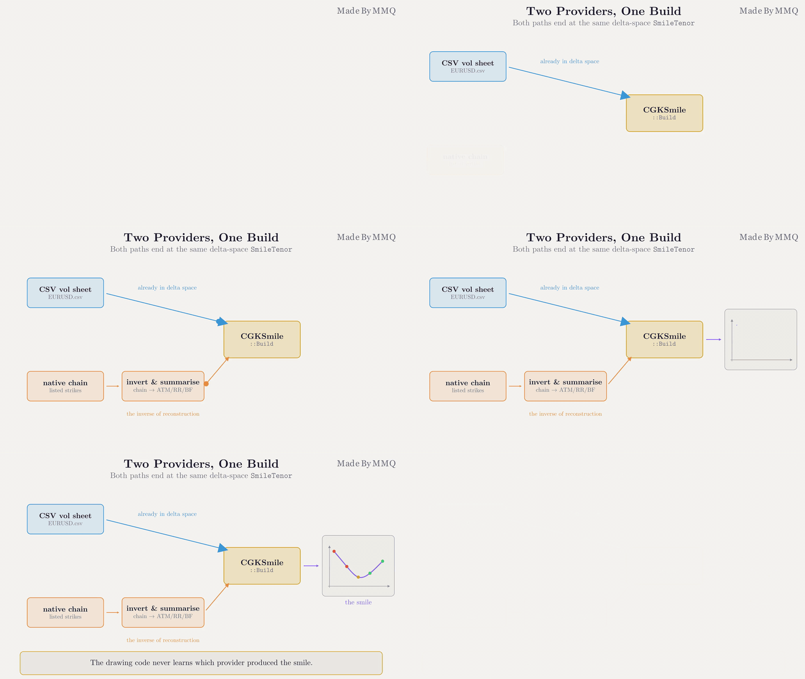
Fig. 5. Two providers, one Build. The CSV path arrives already in delta space; the native path derives delta-space quotes from a listed strike chain.
The Smile Indicator: Drawing and Running It
Everything so far produces a set of points; the indicator, GKSmile.mq5, turns them into something you read on the chart. It draws nothing on the price series itself, so it declares zero plots and buffers and renders entirely onto a full-chart bitmap using the standard-library CCanvas. The inputs let you pick the data source, set the delta and ATM conventions for the pair, choose the x axis, and select the active tenor:
input ENUM_GK_SOURCE InpSource     = GK_SOURCE_CSV;         // data source
input string         InpCsvFile    = "GK\\EURUSD.csv";      // CSV vol sheet (in MQL5\Files)
input string         InpUnderlying = "";                    // native: base symbol (empty = chart symbol)
input ENUM_GK_DELTA  InpDeltaConv  = GK_DELTA_SPOT;         // delta convention (per pair!)
input ENUM_GK_ATM    InpAtmConv    = GK_ATM_DNS;            // ATM convention
input double         InpRateDom    = 0.0430;                // native: domestic rate
input double         InpRateFor    = 0.0250;                // native: foreign rate
input ENUM_GK_XAXIS  InpXAxis      = GK_XAXIS_DELTA;        // x axis: delta pillars or strike
input int            InpTenor      = 1;                     // active tenor index (0-based)
input bool           InpShowAll    = true;                  // draw the other tenors faintly
input int            InpRefreshSec = 0;                     // native re-poll seconds (0 = manual, press R)
input ENUM_GK_THEME  InpTheme      = GK_THEME_DARK;         // card / curve theme
The InpDeltaConv input is the one to set with the convention table from earlier in mind: EURUSD wants the unadjusted spot delta, USDJPY the premium-adjusted one. Reloading the data is where the two providers become one code path. Whichever source is chosen fills a SmileTenor array, and the same Build reconstructs it:
//+------------------------------------------------------------------+
//| (Re)load the chosen data source and reconstruct the smile under  |
//| the selected delta and ATM conventions. Clamps the active tenor  |
//| to the range the data actually carries.                          |
//+------------------------------------------------------------------+
bool Reload(void)
  {
   SmileTenor raw[];
   bool ok = false;
   if(InpSource == GK_SOURCE_CSV)
     {
      CGKProviderCSV csv;
      ok = csv.Load(InpCsvFile, raw);
     }
   else
     {
      string under = (InpUnderlying == "") ? _Symbol : InpUnderlying;
      CGKProviderNative nat;
      ok = nat.Load(under, InpRateDom, InpRateFor, InpDeltaConv, raw);
     }
   if(ok)
      ok = g_smile.Build(raw, InpDeltaConv, InpAtmConv);
   g_haveData = ok;
   if(g_haveData)
     {
      g_active = InpTenor;
      if(g_active < 0)
         g_active = 0;
      if(g_active >= g_smile.NTenors())
         g_active = g_smile.NTenors() - 1;
     }
   return(g_haveData);
  }
The canvas is a bitmap label the size of the chart, created by BuildCanvas in ARGB_RAW mode so its colours are written directly rather than alpha-blended by the terminal. This is why the palette pre-mixes its translucent tones against the card colour instead of relying on transparency. The bitmap is rebuilt only when the chart's pixel size changes.
Two small mappers project data to pixels. The vertical one is a plain volatility-to-pixel map. The horizontal one carries the x-axis choice: in delta mode the pillars are spaced evenly by index, the classic FX smile look that makes the ATM, risk reversal and butterfly read off the shape; in strike mode they sit at their reconstructed strikes, which is what you want when pricing a level.
//+------------------------------------------------------------------+
//| Plot x-coordinate of a pillar. In delta mode the pillars are     |
//| spaced evenly by index (the classic FX smile look); in strike    |
//| mode they sit at their reconstructed strike.                     |
//+------------------------------------------------------------------+
int PxOf(const int tenor, const int j)
  {
   int np = g_smile.NPoints(tenor);
   double f;
   if(g_xaxis == GK_XAXIS_DELTA)
      f = (np <= 1) ? 0.5 : (double)j / (np - 1);
   else
      f = (g_smile.PtStrike(tenor, j) - g_xMin) / (g_xMax - g_xMin);
   return(g_plotX0 + (int)MathRound(f * (g_plotX1 - g_plotX0)));
  }
Drawing one tenor's smile is then a matter of walking its pillars into pixel arrays, filling the area under the active curve one column at a time so it has no seams, stroking an anti-aliased polyline over the top, and dropping a marker on each pillar coloured by its side. The vertical axis is scaled to the active tenor alone: letting every visible tenor vote on the range stretches it across the term structure and squashes the smile you are reading into a thin band. The cost is that a context line can now run off the box, so those are stroked segment by segment with out-of-range parts dropped rather than clamped into a false flat line along the frame:
//+------------------------------------------------------------------+
//| Draw one tenor's smile as a polyline through its pillars. The    |
//| active tenor is drawn bright with filled wings and labelled dot  |
//| markers; the others (when shown) are faint context lines.        |
//+------------------------------------------------------------------+
void DrawSmile(const int tenor, const bool activeTenor)
  {
   int np = g_smile.NPoints(tenor);
   if(np < 2)
      return;
   int xs[], ys[];
   ArrayResize(xs, np);
   ArrayResize(ys, np);
   for(int j = 0; j < np; j++)
     {
      xs[j] = PxOf(tenor, j);
      ys[j] = YOf(g_smile.PtVol(tenor, j));
     }

//--- the y axis is scaled to the active tenor alone, so a context line
//--- can run off the box.
   if(!activeTenor)
     {
      for(int j = 0; j < np - 1; j++)
        {
         double v0 = g_smile.PtVol(tenor, j);
         double v1 = g_smile.PtVol(tenor, j + 1);
         if(v0 < g_yMin || v0 > g_yMax || v1 < g_yMin || v1 > g_yMax)
            continue;
         g_canvas.LineAA(xs[j], ys[j], xs[j + 1], ys[j + 1], g_faint);
        }
      return;
     }

//--- filled area under the active smile, column by column
   for(int j = 0; j < np - 1; j++)
     {
      for(int x = xs[j]; x <= xs[j + 1]; x++)
        {
         double w = (xs[j + 1] == xs[j]) ? 0.0 : (double)(x - xs[j]) / (xs[j + 1] - xs[j]);
         int y = (int)MathRound(ys[j] + w * (ys[j + 1] - ys[j]));
         if(y < g_plotY1)
            g_canvas.LineVertical(x, y, g_plotY1, g_fill);
        }
     }
   g_canvas.PolylineAA(xs, ys, g_line);

//--- pillar markers, each carrying its own reconstructed numbers
   for(int j = 0; j < np; j++)
     {
      string lab = g_smile.PtLabel(tenor, j);
      uint   c   = (lab == "ATM") ? g_atm : (PillarRight(lab) == OPT_PUT ? g_put : g_call);
      g_canvas.FillCircle(xs[j], ys[j], SC(4), c);
      DrawPillarBox(tenor, j, xs[j], ys[j], c);
     }
  }
The reconstruction's actual output is a set of strikes, and a curve plotted in delta space cannot show them: there the x axis is spelling out pillars, not price levels. So each marker carries its own numbers, the strike we solved for sitting above the vol and delta that produced it. That needs one guard: the outer pillars sit on the frame itself, so a block centred on the marker spills over the axis labels beside it. Measuring the widest line and pulling the block back inside the plot fixes it without moving the marker:
//+------------------------------------------------------------------+
//| The reconstruction result, printed at the pillar it belongs to:  |
//| the strike we solved for, its vol and its delta. Reading a       |
//| strike off a curve whose x axis is delta is impossible, so these |
//| three numbers are what turns the picture into a quotable ladder. |
//| The block sits above the marker unless that would leave the plot,|
//| in which case it flips underneath. In delta mode the x axis      |
//| already names the pillar, so the block carries numbers only and  |
//| the accent colour does the naming; in strike mode it labels      |
//| itself, because there the axis is spelling out strikes instead.  |
//+------------------------------------------------------------------+
void DrawPillarBox(const int tenor, const int j, const int px, const int py, const uint accent)
  {
   bool   needLabel = (g_xaxis == GK_XAXIS_STRIKE);
   int    nLines    = needLabel ? 3 : 2;
   string kTx       = StringFormat("%.4f", g_smile.PtStrike(tenor, j));
   string vTx       = StringFormat("%.2f%%  %+.3f", 100.0 * g_smile.PtVol(tenor, j), g_smile.PtDelta(tenor, j));

//--- The outer pillars sit on the frame itself, so a block centred on the
//--- marker spills over the axis labels beside it. Measure the widest line
//--- and pull the block back inside the plot; the marker still anchors it.
   g_canvas.FontSet("Consolas", SC(11));
   int wide = g_canvas.TextWidth(vTx);
   g_canvas.FontSet("Consolas", SC(13), FW_BOLD);
   wide = MathMax(wide, g_canvas.TextWidth(kTx));
   int half = wide / 2 + SC(4);
   int cx   = px;
   if(cx - half < g_plotX0)
      cx = g_plotX0 + half;
   if(cx + half > g_plotX1)
      cx = g_plotX1 - half;

   bool above = (py - SC(14 + 18 * nLines) >= g_plotY0);
   int  y     = above ? py - SC(12) : py + SC(12);
   int  step  = above ? -SC(18) : SC(18);
   uint va    = above ? TA_BOTTOM : TA_TOP;

   if(needLabel)
     {
      g_canvas.FontSet("Segoe UI", SC(12), FW_BOLD);
      g_canvas.TextOut(cx, y, g_smile.PtLabel(tenor, j), accent, TA_CENTER | va);
      y += step;
     }
   g_canvas.FontSet("Consolas", SC(13), FW_BOLD);
   g_canvas.TextOut(cx, y, kTx, accent, TA_CENTER | va);
   g_canvas.FontSet("Consolas", SC(11));
   g_canvas.TextOut(cx, y + step, vTx, g_textDim, TA_CENTER | va);
  }
The two rate sensitivities sit in the header rather than on a per-pillar row, because they are quoted at the ATM strike alone. That is where the second rho earns its place on screen: the domestic and foreign entries carry opposite signs, and reading them together is the difference between hedging one yield curve and hedging the pair. The risk reversal and butterfly the smile was built from sit on the same line, so the quoted inputs and the reconstructed outputs are visible at once.
One detail is worth stealing for any CCanvas tool: every font size and row spacing goes through a single scale derived from the canvas height rather than a pixel constant. Constant font sizes are the classic canvas mistake, since the card grows with the chart while the type does not, and the author never sees it because their own chart never changed size:
//+------------------------------------------------------------------+
//| Font sizes and row spacings are authored against a 580-pixel-tall|
//| card and scaled from there. Pixel-constant fonts are the classic |
//| canvas mistake: they look right on the chart you developed on    |
//| and shrink into illegibility on a large one, since the card      |
//| grows with the chart while the type does not. The clamp keeps    |
//| both extremes sane.                                              |
//+------------------------------------------------------------------+
int SC(const int base)
  {
   return((int)MathRound(base * g_fs));
  }
A compact term-structure strip along the bottom lists the ATM, risk reversal and butterfly across every tenor, the active one boxed, so the single smile and the cross-tenor view sit on one screen. It is also how you check the convention claim from the previous section without leaving the chart, since stepping the active tenor out to 1Y is what makes the premium adjustment worth more than a rounding error.
The remaining plumbing follows the pattern of the surface tool: OnInit resolves the palette, builds the canvas, loads and draws; a timer re-polls the native source when asked; R reloads, the comma and period keys step through the tenors, and X swaps the horizontal axis between the delta pillars and the reconstructed strikes.
Running it: EURUSD against USDJPY
Attach the indicator with the EURUSD sheet and the unadjusted spot-delta convention, and the 1-month smile comes up with a gentle downward tilt. The reconstructed strikes ladder around the 1.0850 spot, the ATM marker sits near a 0.50 call delta as a delta-neutral straddle should, and the put wing prints a little richer than the call wing, the visible signature of a slightly negative risk reversal:
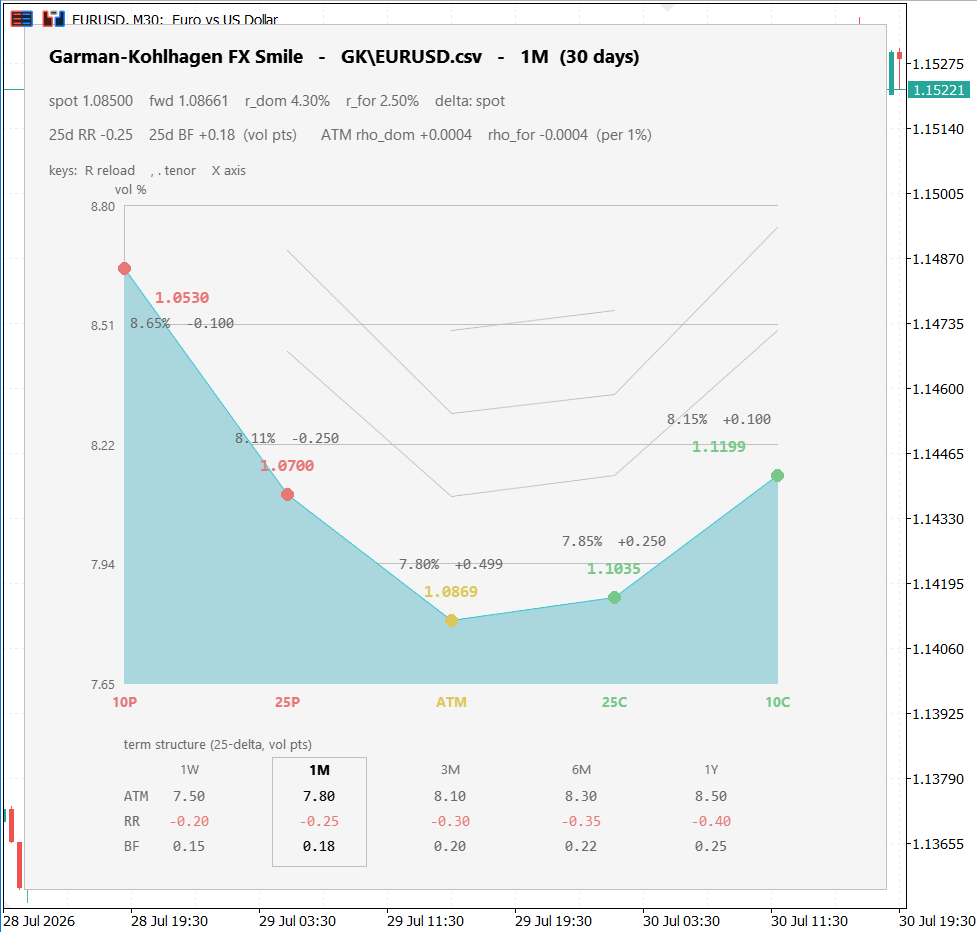
Fig. 6. EURUSD, 1-month. A mild put skew under the unadjusted spot-delta convention, with each pillar carrying its reconstructed strike, vol and delta, and the term structure below.
Now point it at the USDJPY sheet and switch the delta convention to premium-adjusted, as the pair requires. Two things change at once, and they are worth keeping apart. The shape is completely different: a steep, monotonic downward skew, with the 10-delta put printing well above the ATM and the call wing barely lifting. That comes from the sheet's quotes rather than the convention, since USDJPY carries a 25-delta risk reversal of -1.50 against EURUSD's -0.25. What the convention changes is where each pillar lands: the header reports "spot p-adj" in force, and the premium-adjusted ATM strike sits just below the forward, where an unadjusted one would have sat just above:
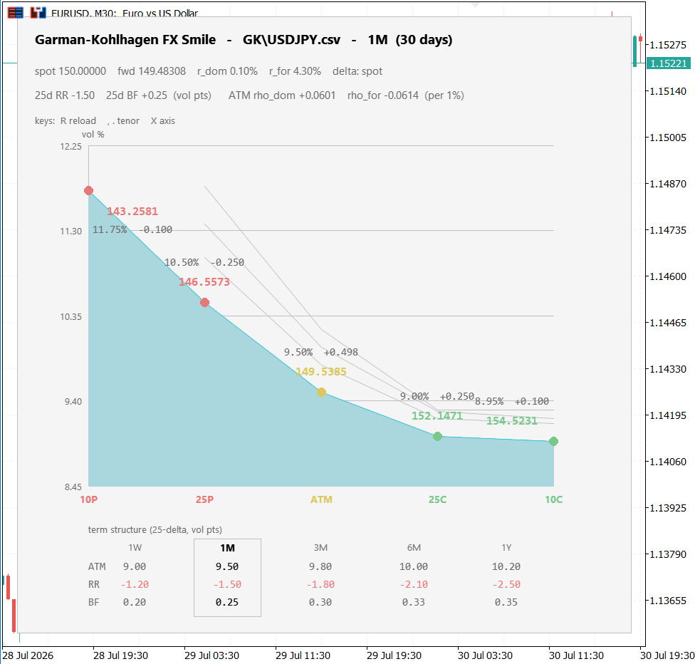
Fig. 7. USDJPY, 1-month, premium-adjusted. A pronounced downside skew, with the convention change visibly relocating the ATM strike relative to the forward.
Reconstructing the two pairs side by side is the article's argument made visible: same code, same input format, the convention set correctly for each, and two smiles a dealer would recognise. Leave USDJPY on the unadjusted delta and the 1-month ladder still reads as a plausible smile, roughly five pips out; step the same mistake to the 1Y tenor and the ATM anchor alone moves by a yen and a half.
Conclusion
We set out to build the FX-native counterpart to a strike-space options tool, and we now have one. Starting from the three numbers an FX desk actually publishes, an at-the-money vol, a risk reversal and a butterfly, the tool prices with Garman-Kohlhagen's two rates, reconstructs the strike-space smile, and draws it with the reconstructed strike ladder on the curve itself, all from either a CSV vol sheet or a broker's native option chain.
The pieces worth carrying away:
- FX is quoted in delta space. The market gives you ATM, risk reversal and butterfly, not a chain of strikes; the strikes are something you reconstruct, and this tool runs that reconstruction. What you get back is a set of pillars, exact where they sit and interpolated in between.
- Garman-Kohlhagen is Black-Scholes with two rates. The foreign rate acts as a continuous yield on the base currency, which gives the two discount factors, the carry-adjusted forward, and a second rho that equity options do not have.
- The delta is a market convention, not a formula. Spot or forward, premium-adjusted or not, fixed per currency pair; reconstructing EURUSD and USDJPY side by side shows how much the choice moves the strikes.
- One reconstruction, two providers. The CSV sheet arrives in delta space; the native chain is summarised into delta space by running the reconstruction backwards, so both feed one engine. That summary is lossy by design, which is why it is a summary and not an inverse.
There is room to build further. The simplified smile-strangle reading could be upgraded to a full market-strangle calibration, or an interpolation model such as SABR or Vanna-Volga could replace the piecewise-linear smile between pillars, letting the tool price arbitrary strikes rather than just the quoted ones. The reconstructed smile is also the natural input to a risk-neutral density, turning the shape into the option market's own distribution for the pair at expiry.
Getting the Source Code via MQL5 Algo Forge
All source files are attached to this article below, but the full repository is also available on MQL5 Algo Forge, the community's Git-based platform for sharing and collaborating on trading projects.
| File name | Description |
|---|---|
| MQL5\Include\GK\GarmanKohlhagen.mqh | Garman-Kohlhagen pricer, the four FX delta conventions, ATM-strike and delta-to-strike solvers, and the full Greeks including both rhos |
| MQL5\Include\GK\GKData.mqh | Smile data structures, the reconstruction engine (ATM/RR/BF to strike pillars), and the CSV vol-sheet provider |
| MQL5\Include\GK\GKProviderNative.mqh | Native option-chain provider: inverts listed contracts and summarises the chain into delta-space quotes, the reconstruction run backwards |
| MQL5\Indicators\GK\GKSmile.mq5 | The chart indicator: delta-space smile with the strike ladder on the curve, plus the term-structure strip, on a CCanvas bitmap |
| MQL5\Files\GK\EURUSD.csv | Sample delta-space vol sheet for EURUSD (unadjusted spot-delta convention) |
| MQL5\Files\GK\USDJPY.csv | Sample delta-space vol sheet for USDJPY (premium-adjusted spot-delta convention) |
Warning: All rights to these materials are reserved by MetaQuotes Ltd. Copying or reprinting of these materials in whole or in part is prohibited.
This article was written by a user of the site and reflects their personal views. MetaQuotes Ltd is not responsible for the accuracy of the information presented, nor for any consequences resulting from the use of the solutions, strategies or recommendations described.

 Practical Modules from Other Languages in MQL5 (Part 07): The OS Module from Python
 Uncertainty as a Model (Part 1): Random Variables — The Language of Uncertainty
 Building AI-Powered Trading Systems in MQL5 (Part 11): Optimizing the UI with Frame Throttling and Partial Rendering
 Building a Swing-Based Volume Profile Indicator in MQL5

- Free trading apps
- Over 8,000 signals for copying
- Economic news for exploring financial markets
You agree to website policy and terms of use