

Neural Networks in Trading: A Unified View of Space and Time (Extralonger)
 82
82
 0
0

Introduction
Predicting the behavior of complex systems has traditionally been one of the key tasks of data analysis. The quality and depth of forecasts determine not only researchers’ academic interest but also very practical outcomes: optimizing flows, reducing costs, and managing risks. This problem is most evident in two areas that might seem unrelated — intelligent transportation systems and financial markets. At first glance, roads with their flows of cars and exchnages with their flows of orders have little in common. However, a closer look reveals a profound structural similarity.
In transportation research, the data form a network in which the nodes are monitoring stations and the edges represent the connections between them. In the financial world, assets, exchanges, brokers, and trading platforms play a similar role, with information and capital circulating continuously among them. If, in a road network, traffic is the signal, then in financial systems such signals are prices, volumes, liquidity, and the behavior of market participants. In both cases, the goal is to identify patterns in spatiotemporal dynamics by analyzing historical data and to make predictions for the future.
Traditional approaches to solving such problems were based on considering the spatial and temporal components separately. In transportation research, this meant analyzing traffic time series separately from the topology of the road network. In finance, similar methods focused either on the temporal dynamics of price series or on structural correlations between assets. This disconnect between space and time creates significant limitations: algorithms become excessively resource-intensive, and their ability to make long-term predictions declines sharply.
The main challenge is that processing temporal features requires repeated iterations over spatial relationships. At the same time, analyzing the structural dependencies between nodes requires multiple passes along the time axis. As a result, the computational complexity becomes an order of magnitude higher than in pure time-series forecasting problems. If we add to this the rapidly growing volumes of data characteristic of transportation systems and financial markets, it becomes clear that without a fundamentally new approach, it is practically impossible to move beyond a horizon of a few hours or a few steps.
One possible solution to this problem was proposed by the authors of the paper "Extralonger: Toward a Unified Perspective of Spatial-Temporal Factors for Extra-Long-Term Traffic Forecasting". The authors draw inspiration from Albert Einstein's ideas about the inseparability of space and time, arguing that spatial and temporal factors must be considered inseparably and simultaneously. This idea is embodied in the concept of Unified Spatial-Temporal Representation — a unified spatial-temporal representation that eliminates the need to artificially separate data into temporal and spatial components. Spatial information is included in each time step, and temporal information is included at each network node.
In transportation systems, this approach has made it possible, for the first time in history, to extend the forecasting horizon from the usual 2–4 hours to an entire week. For financial markets, the potential is even more impressive. Imagine a model that is capable not only of responding to short-term impulses, but also of making meaningful forecasts over time horizons relevant to strategic trading, risk management, and investment planning. In an environment where even a slight advantage in understanding future price dynamics can lead to significant financial results, the ability to make forecasts based on a unified spatial-temporal representation opens up entirely new horizons.
In addition, the unification of space and time radically reduces computational costs. While in the classical formulation the complexity of algorithms increased rapidly and effectively confined researchers to a short horizon, Extralonger demonstrates a reduction in complexity by an order of magnitude. This means that the algorithms run faster and can be applied in real-world scenarios where response time and resource efficiency are critical. As a result, model training is accelerated hundreds of times, and memory consumption is reduced to levels that make long-term forecasting possible even under conditions of limited infrastructure.
This is particularly important for financial markets. After all, the market consists not only of vast amounts of historical data, but also of a continuous stream of new signals that must be processed in real time. Traditional architectures often stumbled at this very stage. Excessive complexity prevented them from handling long-term planning tasks, forcing them to sacrifice either speed or reliability. And sometimes both. The Extralonger framework demonstrates that such compromises are no longer necessary.
The Extralonger Algorithm
Most existing forecasting models are based on what is known as the classical representation of data.

where T is the time-window length, N is the number of network nodes, C is the number of original features, and D is the dimensionality of the transformed feature space.
In practice, this means that the data is first linearly projected into a fixed-dimensional space and then processed by modules responsible for extracting temporal and spatial information.
A classical architecture typically includes two types of modules: temporal and spatial. They can be combined in different orders — first analyzing time, then space. Or, conversely, one can try to process both dimensions simultaneously. In practice, however, any such decomposition had the same drawback: processing features along one axis required multiple iterations along the other. As a result, computational complexity increased rapidly. For example, for Self-Attention mechanisms, it reached an order of O(NT2 + TN2), with a corresponding increase in memory usage. For financial markets, this means that forecasting over a long horizon becomes extremely resource-intensive. Large volumes of historical quotes and interrelationships between instruments simply overload the system.
Attempts to overcome these limitations have been made before including through convolutional models (CNN). In this case, the data was processed as an image, where one axis corresponds to time and the other to a set of nodes. This approach does indeed make it possible to consider space and time simultaneously, but it has limitations. A convolutional window does not allow the entire picture to be captured, but only local regions. Furthermore, the algorithm's complexity was expressed as O(k2TN), where k is the convolution kernel size, which still limited the ability to extend the horizon.
The Extralonger framework radically changes this situation by introducing the Unified Spatial-Temporal Representation. The essence of the idea is simple: space and time are not separated, but are described in a unified way. To do this, the initial representation X∈RT×N×C is first compressed along the feature dimension, after which two linear projections are applied: one over space and the other over time. As a result, two sets of representations emerge:
- Et ∈ RT×D — each time step contains information about all network nodes,
- Es ∈ RN×D — each node accumulates data for all time steps.
Thus, each observation starts carrying a complete spatial-temporal picture, rather than just a local slice. This is the fundamental difference: while the classical representation relied on individual features, the new one provides holistic coverage.
This approach offers several fundamental advantages at once. First, a reduction in complexity. By eliminating redundant iterations, temporal and spatial dependencies are now handled jointly, and the algorithm's complexity is reduced to O(T2 + N2). This makes it possible to make predictions dozens or even hundreds of steps ahead without hitting the limit of computational resources.
Second, simultaneous aggregation. While classical methods were forced to move along a single axis, gradually pulling in information from the other, Extralonger allows each node to be connected to all the others at once at any time step. Consequently, the algorithm is capable of simultaneously accounting for the interactions between different instruments and the dynamics of their changes over time, which is extremely important for a comprehensive analysis of correlations and intermarket relationships.
And finally, third, full receptive-field coverage. By using Self-Attention within a unified representation, Extralonger ensures that every node is connected to every other node at all times. This allows the model to capture the longest-range dependencies — from daily and weekly cycles to more complex patterns associated, for example, with seasonality in the stock market or multi-day trend phases. By comparison: in RNNs, Attention mechanisms, or classical Transformer models, aggregation occurs along separate dimensions, while CNNs are limited to a local receptive window.
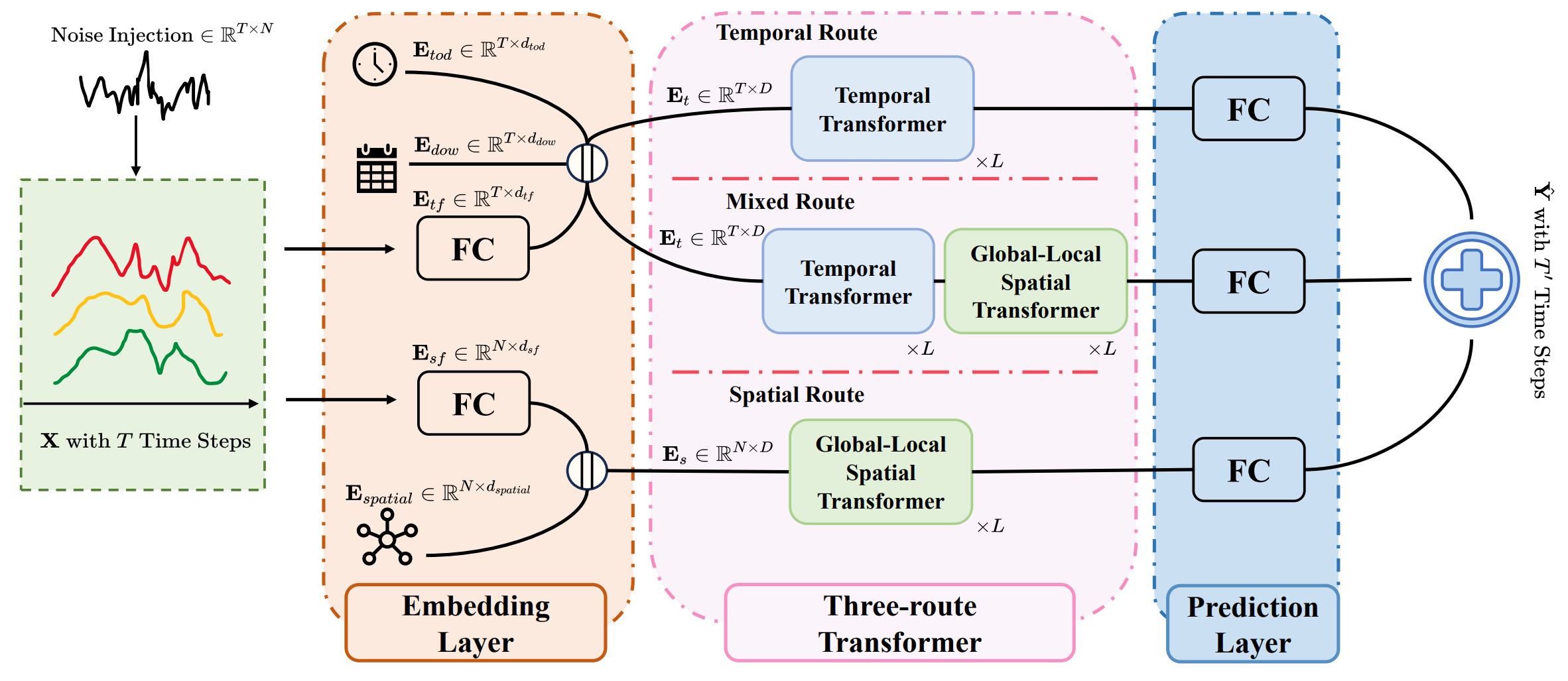
The Extralonger architecture consists of three main components:
- the embedding layer,
- the three-route Transformer module
- forecasting layer.
The embedding layer transforms the input data into an internal representation that includes two key elements: the spatial Es and temporal Et representations. A distinctive feature of the architecture is that data undergoes preprocessing as soon as it enters the system. Learnable noise is introduced into the input data set X, which helps improve the model's resilience to market noise-induced fluctuations.
Next, two fully connected linear projections are applied: one forms temporal features Etf ∈ RT×dtf, and the other forms spatial features Esf ∈ RN×dsf.
In order to capture the cyclical nature inherent in real-world processes, learnable periodicity embeddings have been added to the Extralonger architecture. For the temporal axis, the timestamp-of-day embedding Etod ∈ RT×d_tod is used, reflecting the daily cycle, along with the day-of-week embedding Edow ∈ RT×d_dow, which models weekly seasonality. Similarly, for the spatial dimension, a learnable embedding Espatial ∈ RN×d_spatial is introduced, making it possible to capture stable spatial patterns.
The final representations are obtained by concatenating these embeddings:
- a temporal representation Et = Etf ‖ Etod ‖ Edow ∈ RT×D,
- a spatial representation Es = Esf ‖ Espatial ∈ RN×D.
Thus, fundamental cycles and spatial relationships are incorporated into the model as early as the stage when features are being formed. This is particularly valuable for financial markets: daily fluctuations in liquidity, weekly patterns of activity, and correlations between instruments and trading venues are immediately reflected in the data structure.
At the heart of the system is a three-route Transformer, in which three routes — temporal, spatial, and mixed — operate in parallel. By using a unified spatial-temporal representation, all three routes are able to simultaneously account for both the temporal and spatial structure of the data. At the same time, each route focuses on its own objective. The temporal Transformer in the purely temporal and mixed routes is implemented as a standard Transformer encoder, whereas the spatial route and the mixed route are supplemented with a special module — the Global-Local Spatial Transformer — which allows both local and global relationships to be captured effectively.
Unlike the standard Self-Attention mechanism, in which all network nodes are processed in the same way and without taking their actual structure into account, the Global-Local Spatial Transformer is specifically designed to utilize the topological features of the system under study. In a transportation problem, this refers to a road network in which some stations are connected directly, while others are connected only indirectly. In the world of finance, a similar structure manifests itself in the form of an asset graph: some securities are strongly correlated with one another, while others are linked only through global market trends.
A traditional Transformer treats all connections as equivalent. This makes it possible to capture the overall picture, but at the same time leads to the blurring of local features. Conversely, models that focus exclusively on local connections capture details well but lose the ability to see long-range dependencies. This is precisely where the need for balance arises — taking both global and local patterns into account at the same time.
The GLST module implements this idea directly by combining two attention mechanisms — global and local. In the first stage, the Query, Key, and Value matrices are constructed from the spatial representation Es. Based on these matrices, the global attention coefficients are computed.
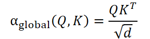
This matrix reflects the strength of the connections between all nodes at once. In a financial context, this can be understood as a matrix of cross-correlations between instruments.
Next, local attention comes into play. To construct it, the adjacency matrix A is used, which defines the structure of the actual connections. In transportation problems, A represents road connections; in finance, however, such a matrix can be a graph of stable correlations or a network of interdependencies among financial instruments. Using A limits attention to neighboring nodes only, creating a local component.

where ⊙ denotes the element-wise product.
Thus, the global component captures broad relationships, while the local component focuses on the closest and most significant connections.
Both matrices undergo SoftMax normalization and are combined into a single expression.

The result is a balanced aggregation in which each node receives information about both the entire system and its immediate connections at the same time.
After that, in the spirit of the classic Transformer, a normalization layer, residual connections (skip-connection), and a Feed-Forward network are applied. These steps form the final updated spatial representation Ês.
It is important to emphasize that this module is particularly well-suited to financial markets. Correlations between assets change over time; the relationships between instruments can be stable or dynamic. The use of global-local attention gives the model flexibility: it can adapt to the current market structure, distinguish between stable and transient relationships, and thus generate a more reliable forecast.
As a result, the Global-Local Spatial Transformer serves as a bridge of sorts between the micro- and macro-levels of analysis. At the micro level, it monitors local market signals and short-term relationships. At the macro level, it identifies global trends and long-term correlations. The combination of these two perspectives makes the model theoretically robust and applicable in real-world trading, where it is precisely the combination of details and the broader context that determines the success of strategies.
Once the three-route Transformer finishes processing the data and generates spatial-temporal representations, the final stage begins: prediction. Its task is to convert abstract embeddings into specific forecast values over a given planning horizon.
To do this, linear projections are used to map the output tensors from the hidden space back into the forecast format. Since the problem formulation in Extralonger is asymmetric (T → T′) — that is, the length of the historical window T and the length of the forecast interval T′ are not the same — it is necessary to explicitly project the Transformer outputs to the dimension T′. In other words, from a historical data segment of a fixed length, we obtain a forecast for a longer or shorter time horizon, which is particularly important for financial markets, where the size of the window can be adjusted depending on the strategy.
After the projection, the results of all three routes (temporal, spatial, and mixed) are combined. Here, the framework's authors do not learn the weights automatically, but instead use a predefined combination — manual tuning of the weighting coefficients. This approach allows us to explicitly adjust the contribution of each route to the final forecast: if desired, we can emphasize the role of the temporal component for markets with pronounced trends or, conversely, focus on spatial dependencies if the structure of correlations between assets is more important.
Taken together, the proposed architecture turns Extralonger into a powerful tool, where each module reinforces the others. The temporal route captures extended dynamics in quotes and volumes, the spatial route captures interdependencies between assets and markets, and the mixed route integrates both aspects, providing a comprehensive view of the market picture.
The authors' visualization of the Extralonger framework is shown below.
Implementation with MQL5
After reviewing the theoretical aspects of the Extralonger framework, we will move on to the practical part of our work, where we will attempt to recreate one possible implementation of its algorithms using MQL5. The advantage of the architecture proposed by the authors lies in its modularity. Each component can be isolated, tested, and, if necessary, replaced or modified. This is particularly valuable for trading systems, where flexibility and the ability to adapt to the specific characteristics of particular markets are important. In our case, we will also take a step-by-step approach — module by module — making the most of the set of objects we have already developed to avoid duplicating functionality.
As noted in the theoretical section, the processing of the raw data begins with the addition of learnable noise. It is important to note, however, that “noise” here does not refer to the traditional random component generated by pseudorandom number generators. On the contrary, this is a matrix of learnable parameters that acts as an additional offset. In other words, this is not a random distortion, but a deliberate expansion of the feature space that allows the model to capture hidden relationships that are not apparent in the original data.
If we draw an analogy with classical architectures, this layer performs the same function as learnable positional encoding in Transformer models. There, it allows the model to distinguish between positions in a time series; here, it adds the ability to shift the data in a direction that facilitates the subsequent identification of patterns. And it is precisely this quality that makes the approach particularly valuable for financial markets: such shifts may in fact encode stable seasonal patterns or weak correlations that are not directly reflected in the price series.
Our library already contains the CNeuronLearnabledPE object, which performs similar functionality. Its purpose is to add a learnable positional offset to the input data, and in the context of implementing the Extralonger framework, it is a perfect fit for the task of learnable noise. Essentially, we can use a ready-made, time-tested solution without having to invent a new component.
Not only does this save effort, but it also ensures reliability, since the object has been tested in previous experiments.
The next step after adding the learnable offset is to form projections in the temporal and spatial planes. In the theoretical description of the Extralonger framework, two fully connected layers are used for this purpose; working in parallel, they generate two sets of embeddings.
In our implementation, we can delegate this task to the CNeuronConvOCL convolutional layer objects. This solution is natural and convenient. Convolution operations have already proven themselves to be a versatile tool for transforming input arrays. They make it easy to control the number of input and output channels by specifying the kernel size. Consequently, the formation of temporal and spatial projections can be implemented as two parallel convolutional layers: the first operates along the time axis and forms Et, while the second operates along the node axis and forms Es. This fully aligns with the idea of the authors of Extralonger while preserving the uniformity of our implementation.
Adding Spatial Embeddings
Next comes the stage of adding spatial and temporal embeddings. At first glance, there are no particular difficulties here. We have encountered similar operations before. Creating a spatial embedding with a fixed data structure is similar to the previous step of adding learnable noise. However, at this stage, we do not sum the tensors; instead, we concatenate them, combining information from different sources. The process is implemented in the new CNeuronSpatialEmbedding object, which inherits the core functionality from CNeuronBaseOCL and extends it to suit our needs.
class CNeuronSpatialEmbedding   :     public CNeuronBaseOCL
  {
protected:
   uint              iWindow;
   uint              iUnits;
   uint              iEmbeddingDim;
   CParams           cEmbedding;
   //---
   virtual bool      feedForward(CNeuronBaseOCL *NeuronOCL) override;
   virtual bool      updateInputWeights(CNeuronBaseOCL *NeuronOCL) override;
   virtual bool      calcInputGradients(CNeuronBaseOCL *NeuronOCL) override;

public:
                     CNeuronSpatialEmbedding(void) {};
                    ~CNeuronSpatialEmbedding(void) {};
   //---
   virtual bool      Init(uint numOutputs, uint myIndex, COpenCLMy *open_cl,
                          uint units, uint window, uint embed_dim,
                          ENUM_OPTIMIZATION optimization_type, uint batch);
   //---
   virtual int       Type(void)   const   {  return defNeuronSpatialEmbedding;   }
   //--- methods for working with files
   virtual bool      Save(int const file_handle) override;
   virtual bool      Load(int const file_handle) override;
   //---
   virtual bool      WeightsUpdate(CNeuronBaseOCL *source, float tau) override;
   virtual void      SetOpenCL(COpenCLMy *obj) override;
   virtual void      SetActivationFunction(ENUM_ACTIVATION value) override { };
  };
The neuron's architecture is defined in the Init initialization method. This is where its key parameters are specified: the number of individual sequences, the size of each one, and the embedding dimension.
bool CNeuronSpatialEmbedding::Init(uint numOutputs, uint myIndex, COpenCLMy *open_cl,
                                   uint units, uint window, uint embed_dim,
                                   ENUM_OPTIMIZATION optimization_type, uint batch)
  {
   if(!CNeuronBaseOCL::Init(numOutputs, myIndex, open_cl, (window + embed_dim)*units,
                                                           optimization_type, batch))
      return false;
   activation = None;
Inside the method, the parent neuron class with OpenCL support is initialized first. The dimension of the result tensor is calculated as the sum of the unitary-sequence representation length and the embedding dimension, multiplied by the number of such sequences. If the base initialization fails, the method terminates correctly and returns an error signal.
Next, the neuron configures the activation function, although it is not yet used by the neuron itself.
Next, we initialize the embedding generation object. Here, we use the hyperbolic tangent TANH as the activation function; it introduces nonlinearity and constrains the values to the range [-1, 1]. This helps the model form more robust representations of market patterns and prevents extreme values from having an excessive influence on the learning process.
   if(!cEmbedding.Init(0, 0, OpenCL, embed_dim * units, optimization, iBatch))
      return false;
   cEmbedding.SetActivationFunction(TANH);
//---
   iUnits = units;
   iWindow = window;
   iEmbeddingDim = embed_dim;
//---
   return true;
  }
The neuron's parameters are then saved for subsequent forward and backward passes.
As a result, the Init method seamlessly bridges theory and practice. The neuron becomes fully ready to process data, concatenate embeddings, and pass on structured information. This provides a solid foundation for building trading models that can analyze market signals across different time horizons and identify hidden dependencies that are important for making informed trading decisions.
The feedForward method implements the algorithm for the forward pass of data through the neuron — from inputs to outputs. In a financial context, this is similar to how a trader systematically analyzes historical data and forms an integrated representation of the current market situation.
First, the system checks whether the pointer to the previous NeuronOCL neuron is valid. If it does not exist, the method immediately returns false. This is important. Without source data, a forward pass is impossible, just as it is impossible to make decisions without market quotes.
bool CNeuronSpatialEmbedding::feedForward(CNeuronBaseOCL *NeuronOCL)
  {
   if(!NeuronOCL)
      return false;
Next, if the neuron is in training mode (bTrain=true), a forward pass is performed on the cEmbedding object. This is where spatial embeddings are generated, encoding key market dependencies within the selected data window. If this operation fails, the method returns false to indicate a problem with creating the embeddings.
   if(bTrain)
      if(!cEmbedding.FeedForward())
         return false;
Please note that this operation is performed only during the training process. After all, in this case, the embeddings do not depend on the source data, but merely encode the positions of the sequences. Consequently, the values remain fixed during operation, and we eliminate unnecessary operations, which will speed up the decision-making process.
Once the embeddings have been generated, the next key step is to concatenate the source data with the embeddings. The Concat method combines the outputs of the previous neuron and the embedding into a single Output tensor, taking into account the representation size of each unitary sequence and the embedding dimension.
   if(!Concat(NeuronOCL.getOutput(), cEmbedding.getOutput(), Output, iWindow, iEmbeddingDim, iUnits))
      return false;
//---
   return true;
  }
Finally, if all operations were successful, the method returns true, indicating that the neuron's forward pass was completed correctly and the result tensor is ready to be passed to the next layer of the model.
As you can see, the algorithm for the forward pass method is quite simple and organized in a linear fashion. It sequentially checks the input data, generates spatial embeddings, and concatenates them with the outputs of the previous layer, creating a tensor ready to be passed on. Backward pass methods are structured similarly, following the same pattern but in the opposite direction. Thanks to this clear and consistent structure, both methods are easy to understand and allow you to focus on the key features of how a neuron processes time series of financial data.
For a more in-depth study, we recommend that you explore the implementation of the backward pass on your own. The complete code of the CNeuronSpatialEmbedding class and all its methods is provided in the attachment, making it possible to trace the neuron's operation from initialization to embedding generation and the transfer of information to the model.
Temporal Embedding
The situation is a bit more complicated when it comes to temporal embeddings. First, there are several of them, and each encodes different temporal cycles. The framework's authors propose using two levels: intraday and intra-weekly. This task is familiar from our previous experiments with the temporal encoder of the HimNet framework, where we also generated embeddings for time series. Back then, recurrent blocks were used, and at each step the input-data tensor received only the embeddings of the state being analyzed.
Now the problem is a little more difficult. At each pass through the neuron, an entire temporal sequence is analyzed, and each of its time steps must receive its own temporal embeddings. This is similar to the work of a trader who does not just look at the current price or an indicator, but simultaneously evaluates a whole range of historical signals to identify hidden cycles and patterns.
We will, of course, use the developments from HimNet, but adapt them to the new architecture, where temporal embeddings are generated simultaneously for all steps in the sequence, allowing the model to capture market dynamics more accurately and respond more appropriately to market changes.
We begin building the temporal embedding algorithm in the OpenCL program, where we create the ConcatByLabel kernel. This kernel performs the task of concatenating the input data with multiple levels of embeddings — in our case, two temporal embeddings corresponding to intraday and intra-weekly cycles. In a financial context, this is similar to analyzing multiple time horizons simultaneously: short-term fluctuations and longer-term cycles all influence the forecast, and the model must take them all into account.
The kernel uses a three-dimensional grid of global identifiers: row_id, col_id, and buffer_id. This allows us to process the rows and columns of the source tensor simultaneously, as well as choose which buffer to work with — the source data or one of the embeddings.
__kernel void ConcatByLabel(__global const float* data,
                            __global const float* label,
                            __global const float* embedding1,
                            __global const float* embedding2,
                            __global float *output,
                            const int dimension_data,
                            const int dimension_emb1,
                            const int dimension_emb2,
                            const int frame1,
                            const int frame2,
                            const int period1,
                            const int period2
                           )
  {
   const size_t row_id = get_global_id(0);
   const size_t col_id = get_global_id(1);
   const size_t buffer_id = get_global_id(2);
   const size_t total_rows = get_global_size(0);
   const size_t total_cols = get_global_size(1);
   const size_t total_buffers = get_global_size(2);
First, each thread is assigned global identifiers:
- row_id — the row index, corresponding to a timestamp or time series step;
- col_id — the column index, corresponding to a specific variable or feature;
- buffer_id — specifies which buffer this thread is working with: the input data, the first embedding, or the second embedding.
The global dimensions of the problem space determine the overall thread grid. It is important to understand here that total_buffers determines how many different datasets we concatenate. The final dimensionality of the output vector is determined accordingly.
   __global const float *buffer;
   int dimension_in, dimension_out;
   int shift_in, shift_out;
//---
   switch(total_buffers)
     {
      case 1:
         dimension_out = dimension_data;
         break;
      case 2:
         dimension_out = dimension_data + dimension_emb1;
         break;
      case 3:
         dimension_out = dimension_data + dimension_emb1 + dimension_emb2;
         break;
      default:
         return;
     }
If there are more than three buffers, the current thread simply returns from the kernel, preventing incorrect use.
The next step is to select a specific buffer and calculate the offsets for reading and writing data.
   switch(buffer_id)
     {
      case 0:
         buffer = data;
         dimension_in = dimension_data;
         shift_in = RCtoFlat(row_id, col_id, total_rows, dimension_in, 0);
         shift_out = RCtoFlat(row_id, col_id, total_rows, dimension_out, 0);
         break;
      case 1:
         buffer = embedding1;
         dimension_in = dimension_emb1;
         shift_in = ((int)IsNaNOrInf(label[row_id] / frame1, 0)) % period1;
         shift_in = RCtoFlat(shift_in, col_id, period1, dimension_in, 0);
         shift_out = RCtoFlat(row_id, dimension_data + col_id, total_rows, dimension_out, 0);
         break;
      case 2:
         buffer = embedding2;
         dimension_in = dimension_emb2;
         shift_in = ((int)IsNaNOrInf(label[row_id] / frame2, 0)) % period2;
         shift_in = RCtoFlat(shift_in, col_id, period2, dimension_in, 0);
         shift_out = RCtoFlat(row_id, dimension_data + dimension_emb1 + col_id, total_rows,
                                                                           dimension_out, 0);
         break;
     }
For the input data, shift_in and shift_out are calculated directly using the RCtoFlat function, which converts the two-dimensional row and column indices into a linear index of the global buffer.
For embeddings, shift_in depends on the timestamp value for the individual sequence step, label[row_id], divided by the period (frame1 or frame2). This allows for the cyclical selection of an embedding that corresponds to a specific phase of the time cycle, which is particularly important for financial data with recurring intraday and intra-weekly patterns.
After the preparatory work is completed, the corresponding data is written to the result buffer.
   if(col_id < dimension_in)
      output[shift_out] = IsNaNOrInf(buffer[shift_in], 0);
  }
It is important to note here that we assume the use of different dimensionalities for the input data and embeddings. When the kernel is enqueued for execution, the maximum parameter value is used; therefore, before performing buffer access operations, we check whether the column index is valid for the buffer being used. In addition, the data is cleaned of invalid values (NaN or Inf) so as not to interfere with subsequent calculations.
As a result, the kernel generates a fully concatenated tensor that takes into account all specified embeddings and the input data. Each time step receives its own set of embeddings, which allows the model to see the entire market dynamics at once—including short-term fluctuations and longer cycles — thereby improving the quality of forecasts and the robustness of trading models.
Once the forward pass algorithm has been developed, the natural next step is to implement the error backpropagation process. While the forward pass generates embeddings and combines them with the input data, the backward pass is responsible for adjusting the weights and improving the quality of information representations. In a financial context, this is similar to the work of a trader who, by evaluating the consequences of past decisions, adjusts their strategy for the next move. Forecast errors at previous time steps allow the model to adjust the embeddings to better reflect market dynamics.
In this case, backpropagation occurs between the input data and the corresponding embeddings. And it is implemented in the ConcatByLabelGrad kernel. Essentially, this is the step in which the network propagates errors back to each component, allowing the weights to be adjusted and the prediction to be improved.
__kernel void ConcatByLabelGrad(__global float* data_gr,
                                __global const float* label,
                                __global float* embedding1_gr,
                                __global float* embedding2_gr,
                                __global float *output_gr,
                                const int dimension_data,
                                const int dimension_emb1,
                                const int dimension_emb2,
                                const int frame1,
                                const int frame2,
                                const int period1,
                                const int period2,
                                const int units
                               )
  {
   const size_t row_id = get_global_id(0);
   const size_t col_id = get_global_id(1);
   const size_t buffer_id = get_global_id(2);
   const size_t total_rows = get_global_size(0);
   const size_t total_cols = get_global_size(1);
   const size_t total_buffers = get_global_size(2);
//---
   __global float *buffer;
   int dimension_in, dimension_out;
   int shift_in, shift_out, shift_col;
   int period, frame, rows;
Initially, each thread is identified in the three-dimensional problem space. This allows a separate thread to process a specific combination of time step, feature, and buffer.
Next, the final dimensionality of the result tensor — in this case, the error gradients — is determined.
   switch(total_buffers)
     {
      case 1:
         dimension_out = dimension_data;
         break;
      case 2:
         dimension_out = dimension_data + dimension_emb1;
         break;
      case 3:
         dimension_out = dimension_data + dimension_emb1 + dimension_emb2;
         break;
      default:
         return;
     }
I think you have noticed the repeated operations from the forward-pass kernel. However, there are differences ahead. If the buffer being processed is the input data (buffer_id == 0), then the gradients are simply copied directly from the error gradient buffer at the output level. After that, we return from the kernel.
   switch(buffer_id)
     {
      case 0:
         if(col_id < dimension_data && row_id<units)
           {
            shift_in = RCtoFlat(row_id, col_id, total_rows, dimension_in, 0);
            shift_out = RCtoFlat(row_id, col_id, total_rows, dimension_out, 0);
            data_gr[shift_in] = IsNaNOrInf(output_gr[shift_out], 0);
           }
         return;
However, in the case of embeddings (buffer_id == 1 or 2), the algorithm is a bit more complex. Here we first determine the period and the offset for which we will collect gradients.
      case 1:
         rows = period1;
         buffer = embedding1_gr;
         dimension_in = dimension_emb1;
         shift_in = RCtoFlat(row_id, col_id, period1, dimension_in, 0);
         shift_col = dimension_data;
         period = period1;
         frame = frame1;
         break;
      case 2:
         rows = period2;
         buffer = embedding2_gr;
         dimension_in = dimension_emb2;
         shift_in = RCtoFlat(row_id, col_id, period2, dimension_in, 0);
         shift_col = dimension_data + dimension_emb1;
         period = period2;
         frame = frame2;
         break;
     }
Next, we check whether the current thread falls within the dimensions of the corresponding embedding in terms of the representation dimension and data periodicity. Only then do we set up a loop that iterates through all the time steps of the error gradient tensor at the output level and accumulates the error contribution for each embedding.
   if(row_id >= rows || col_id >= dimension_in)
      return;
   float grad = 0;
   for(uint r = 0; r < total_rows; r ++)
     {
      int row = ((int)IsNaNOrInf(label[r] / frame, 0)) % period;
      if(row != row_id)
         continue;
         shift_out = RCtoFlat(r, shift_col + col_id, total_rows, dimension_out, 0);
      grad += IsNaNOrInf(output_gr[shift_out], 0);
     }
   buffer[shift_in] = IsNaNOrInf(grad, 0);
  }
In the loop body, we first determine which periodicity object the current step belongs to, so that the gradients are accumulated according to the corresponding phase position of the time cycle. Only if the resulting value matches the element being analyzed do we sum the errors at the output level.
The accumulated error gradient is written to the global gradient buffer for the corresponding embedding. At the same time, do not forget to sanitize the obtained result by removing any invalid values (NaN or Inf).
As a result, the ConcatByLabelGrad kernel accurately distributes errors between the input data and the embeddings, ensuring that weights are updated correctly at all levels of the temporal sequence. This allows the model to adapt to the complex cycles of financial time series, improving forecast accuracy and robustness to noise.
We've put in a lot of work, and the article is already looking quite substantial. I suggest we take a short break so that the information can sink in and we can process it calmly. We will continue the implementation we've started and discuss it in detail in the next article.
Conclusion
In this article, we explored the Extralonger framework, which combines spatial and temporal factors into a single model for forecasting time series. This approach significantly reduces computational complexity and memory requirements compared to traditional methods. This expands forecasting horizons to an unprecedented scale.
The particular value of this approach lies in assigning each element of the time series its own embedding, which allows the model to account for both short-term fluctuations and long-term patterns simultaneously. This principle can be adapted to address a variety of problems where the interaction of spatial and temporal factors is important — from financial markets to urban infrastructure planning or weather forecasting.
Extralonger opens up a new path for building effective forecasting models based on spatial-temporal data, combining high accuracy, resource efficiency, and scalability over long time horizons.
References
- Extralonger: Toward a Unified Perspective of Spatial-Temporal Factors for Extra-Long-Term Traffic Forecasting
- Other articles in this series
Software used in this article
| # | Name | Type | Description |
|---|---|---|---|
| 1 | Study.mq5 | Expert Advisor | Expert Advisor for offline model training |
| 2 | StudyOnline.mq5 | Expert Advisor | Expert Advisor for online model training |
| 3 | Test.mq5 | Expert Advisor | Model testing Expert Advisor |
| 4 | Trajectory.mqh | Class Library | Structure describing the system state and model architecture |
| 5 | NeuroNet.mqh | Class Library | Class library for building a neural network |
| 6 | NeuroNet.cl | Library | Code library for an OpenCL program |
Translated from Russian by MetaQuotes Ltd.
Original article: https://www.mql5.com/ru/articles/19494
Warning: All rights to these materials are reserved by MetaQuotes Ltd. Copying or reprinting of these materials in whole or in part is prohibited.
This article was written by a user of the site and reflects their personal views. MetaQuotes Ltd is not responsible for the accuracy of the information presented, nor for any consequences resulting from the use of the solutions, strategies or recommendations described.

 Features of Custom Indicators Creation
 Artificial Searching Swarm Algorithm (ASSA)
 Features of Experts Advisors
 Building a Neural Loss-Pattern Auditor in MQL5

- Free trading apps
- Over 8,000 signals for copying
- Economic news for exploring financial markets
You agree to website policy and terms of use