MetaTrader 5 Machine Learning Blueprint (Part 21): Feature Importance Analysis

Table of Contents

1. Introduction
2. Why One Importance Column Is Not Enough
3. An Experiment Where the Answer Is Known in Advance
4. How Far One Signal's Credit Spreads
5. The Two Clustered Methods Disagree
6. Single Feature Importance Measures Something Else
7. Wiring the Analysis into the Training Run
8. Reading the Report
9. Conclusion
10. Attached Files

Introduction

A trained model in this series ends its run by averaging the feature_importances_ of every tree in its ensemble and sorting the result. That column answers one narrow question: across the training set, which columns did the trees split on most productively? It is in-sample, it is specific to tree-based learners, and it has a property that becomes a problem the moment a feature set grows past a handful of columns. Two features carrying the same information are interchangeable at every split, so each is chosen about half the time, and each receives about half the credit.

That is not a rounding error. Engineer one predictor six ways and its six copies can each land below features that carry a fraction of the information, while the ranking looks entirely reasonable. Nothing in the output flags it. The ranking is not wrong about what the trees did; it is wrong about what the features are worth.

López de Prado sets out the diagnosis and three corrections in Advances in Financial Machine Learning (AFML) chapter 8, and a fourth in Machine Learning for Asset Managers (MLAM) section 6.5.2. This article measures the problem on data where the right answer is fixed by construction, then applies each correction and reports which ones recover it. Two of them disagree with each other, and the disagreement is a property of the methods rather than of the data.

Why One Importance Column Is Not Enough

Mean Decrease Impurity

MDI accumulates, for every split in every tree, how much impurity that split removed, and attributes it to the splitting feature. It is cheap, because the quantity is already computed during fitting. It is also in-sample, it applies only to tree ensembles, and it assigns every feature some importance whether or not the feature carries information.

The dilution follows from how a split is chosen. A node picks one column and one threshold. If two columns encode the same quantity, both separate the node about equally well, so the tie between them is broken close to arbitrarily. The impurity removed is the same whichever column wins, but it is booked entirely to the winner. Over an ensemble, each of the two columns wins about half the time and each is credited with about half of what the underlying quantity is worth.

Snippet 8.2 recommends fitting the importance model with max_features=1. With one candidate feature per split, the trees cannot systematically prefer one member of a correlated group over another, which removes masking. It does not remove dilution. Masking is one feature crowding out another; dilution is one feature's credit being divided. The first is a bias in which column gets picked, the second is a consequence of any column having to be picked at all.

Mean Decrease Accuracy

MDA fits the model on each training fold, scores the held-out fold, then permutes one column at a time and re-scores. The importance of a column is the degradation its permutation causes. This works for any classifier and it is measured out of sample, which makes it the more trustworthy of the two. The cross-validation must be purged and embargoed, since overlapping triple-barrier labels leak across an ordinary fold boundary.

MDA is still susceptible to substitution, and in a way that is worse than MDI's. Permuting a column destroys the information in that column only. If an identical second column is still intact, every tree that split on the second one is unaffected, and the trees that split on the permuted one can be compensated for by the rest of the ensemble. The score barely moves, so both columns are reported as unimportant. Under MDI a duplicated predictor is understated; under MDA a duplicated predictor can be erased entirely.

Clustered Impurity and Accuracy

Section 6.5.2 of MLAM proposes grouping features by dependence and scoring the groups. Clustered MDI sums the member impurities within each cluster. Clustered MDA permutes every column in a cluster together, so there is no surviving copy for the model to fall back on. Both then broadcast the cluster's score to each of its members, which means every member of a cluster ends up with an identical number.

The clustering itself is done by ONC, optimal number of clusters, which searches for the number of clusters maximizing the t-statistic of the silhouette scores. It is unsupervised: it sees the dependence structure of the feature matrix and never sees the labels. That independence is what makes the correction honest, and it is also the reason the partition has to be inspected rather than trusted, since a metric that misses a relationship will leave substitutes in separate clusters.

This is the same machinery Part 20 built, and the correlation matrix it consumes is the object Part 20 spent its length cleaning. The connection is structural rather than decorative. ONC clusters a distance matrix derived from a sample correlation matrix. A correlation estimated from T observations of N features contains noisy eigenvalues, whose spread the Marčenko–Pastur law predicts from T/N alone. Any remaining noise affects the partition. That partition, in turn, determines all clustered scores reported in this article. Clustering on a raw correlation matrix therefore discards the result Part 20 established.

Before ONC, we apply Part 20's correction. We fit the Marčenko–Pastur density to the empirical eigenvalue distribution, estimate the noise ceiling, keep eigenvalues above it, and replace those below it with their common average to preserve the trace. The rebuilt matrix has the same leading structure and a flat noise floor.

One parameter of that fit does more work than the rest. The ceiling depends on observations per variable, and a panel of persistent features does not carry one independent observation per row. Part 20's AR(1) effective-sample-size correction replaces T with T(1-ρ)/(1+ρ). On the matrix used here the average lag-1 autocorrelation is 0.764, which turns 1,470 rows into 197 effective observations and drops q from 33.4 to 4.48. The noise ceiling rises from 1.376 to 2.169 and the number of eigenvalues treated as signal falls from eight to five. Skipping the correction leaves three noise eigenvalues protected from shrinkage.

Single Feature Importance

SFI sidesteps substitution entirely by fitting a separate model on each feature in isolation and reporting its cross-validated score. With one column there is nothing to substitute for. The cost is that joint effects vanish: a feature useful only in combination with another scores as though it were useless, and a feature that is valuable for explaining the splits of a second feature gets no credit at all.

An Experiment Where the Answer Is Known in Advance

Measuring dilution requires knowing what the undiluted answer should be. The synthetic market used here is built around a slow AR(1) latent state that drives the drift of the next bar, with stochastic volatility layered on so the triple barrier has something to adapt to. The latent state is genuinely predictive of the next move and far from deterministic.

Four feature sources are supplied to the pipeline. The first re-expresses the latent state six ways: a noisy copy, an exponentially weighted version, a rolling percentile rank, a hyperbolic tangent, a clipped copy, and a smoothed slope. Every one is a monotone or near-monotone transform of the same quantity, which is exactly the situation an indicator library produces when several of its members read the same underlying market state. The second source contributes a single unduplicated momentum feature. The third contributes ordinary price and volatility columns, and the fourth eight columns of pure noise. The pipeline appends its own calendar and session block, bringing the matrix to 44 columns.

Labels come from the same triple-barrier machinery a model would be trained against, and the sample weights from the same weighting-scheme search, so the importances are measured against the labels and weights a real training run would see. After aligning features to events and dropping warm-up rows, 1,470 events survive. The importance model is a random forest with max_features=1, reaching an out-of-bag score of 0.9442 and a cross-validated negative log-loss of -1.0025 under the selected weighting scheme.

The ground truth is therefore fixed before any importance method runs. Six columns carry one signal. One column carries a weaker independent signal. Eight carry nothing, and the calendar block the pipeline adds carries nothing either, since the synthetic market has no session structure to find.

How Far One Signal's Credit Spreads

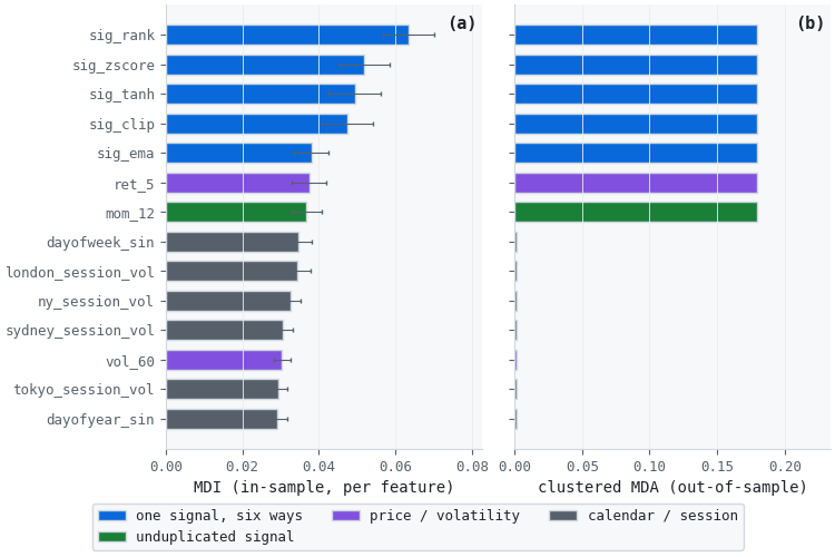
Figure 1. Two-panel illustration of one signal's credit split across six engineered copies

• Panel (a): the seventeen highest-scoring features under per-feature MDI. Five of the six copies of the latent signal hold the top five places, scoring 0.0381 to 0.0635. The sixth, sig_slope, is last in the panel at 0.0250, below eleven features that are not copies of anything.
• Panel (b): the same seventeen features scored by clustered MDA. Nine of them make up the signal-bearing cluster and carry its single score of 0.1927. The rest carry 0.0019.
• Bottom bar of each panel: sig_slope is the clearest reading of the correction. It sits last under per-feature MDI and at full length under clustered MDA, because the cleaned correlation matrix places it with its siblings.
• Scales: the panels measure different quantities and share only their feature list. Panel (a) is a share of a budget summing to one across all 44 columns; panel (b) is out-of-sample log-loss degradation. Bars are comparable within a panel, not across the pair.

Panel (a) puts a number on the dilution. The six copies score 0.0635, 0.0519, 0.0495, 0.0475, 0.0381 and 0.0250, and they sum to 0.2755. The best of the eight pure-noise columns scores 0.0152. Because MDI is normalized so the whole column sums to one, these are shares of a fixed budget, and adding the shares of six columns that encode one quantity is a fair estimate of what that quantity is worth to the model: roughly eighteen times the best noise column.

No single copy comes close to that figure. The strongest is worth about four noise columns, the weakest about 1.6. Sixteen features rank above sig_slope. Five of them are its own siblings and three carry real information, but the remaining eight are seven calendar features and one volatility feature, none of which knows anything about the direction of the next move. A ranking that seats eight uninformative columns above a genuine predictor is not a ranking anyone can safely prune on.

The point worth being precise about is that panel (a) does not look broken. Its top is occupied by features that genuinely matter, its bottom by features that genuinely do not, and the ordering in between reads like a plausible result. A practitioner cutting the bottom half of the full table deletes sig_slope and keeps london_session_vol. The method has not produced an obviously wrong answer, it has produced a quietly wrong one, and nothing in its output distinguishes the two cases.

Panel (b) is what happens when the copies are permuted together instead of one at a time. ONC placed all six in a single cluster, along with the momentum feature and two return columns, and put the remaining 35 features in a second cluster. Destroying the first cluster costs the model 0.1927 in held-out log-loss; destroying the second costs 0.0019. The gap between what matters and what does not widens from about four to one under naive MDI to about 100 to one here, for a mechanical reason: with every copy shuffled at once, the model has nothing left to read the latent state from.

That all six copies land together is a consequence of the cleaning step, not a given. sig_slope is a smoothed four-bar difference of the latent state, so it tracks the state's rate of change rather than its level, and its raw linear correlation with the level is weak enough to be indistinguishable from the noise band. Clustering the raw sample correlation puts it with the noise, in a cluster of 36, where it keeps its diluted score of 0.0250 and the correction never reaches it. Shrinking the noise eigenvalues first raises it above that band, and the partition becomes 35 and 9 with every copy in the informative group.

Detoning is available on the same call and is left off by default here, on evidence rather than preference. Removing the leading eigenvector is standard when the first mode is a market factor shared by every asset in a portfolio. In a feature panel built around one predictor, the leading mode is the predictor, and stripping it merges the signal group into a 31-member cluster that no longer isolates anything. Detone when the first eigenvector represents something the analysis wants to control for; leave it off when it represents what the analysis is looking for.

The Two Clustered Methods Disagree

Both clustered methods ran on the identical ONC partition. They ranked it in opposite orders.

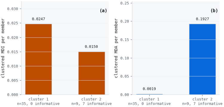
Figure 2. Two-panel illustration of clustered impurity and clustered accuracy on an identical partition

• Panel (a): clustered MDI. The 35-member cluster scores 0.0247 per member against 0.0150 for the 9-member cluster that carries the signal, so the ordering is inverted.
• Panel (b): clustered MDA on the same partition, separating the two clusters by a factor of 100.6 in the correct direction.

Cluster	Members	Clustered MDI	Clustered MDA
Noise-dominated	35	0.0247	0.0019
Signal-bearing	9	0.0150	0.1927

The cause is arithmetic, not statistical. The steps are as follows. Clustered MDI first sums the impurity of a cluster's members. It then writes that one sum onto every member of the cluster as that member's score. Finally, it normalizes the entire column to sum to one. The normalization is where the size enters: a 35-member cluster writes its total into the column 35 times, while a 9-member cluster writes its total only 9 times, so the larger cluster dominates the denominator that both are divided by. Each member's published figure ends up proportional to its own cluster's raw total, and raw totals reward size. Thirty-five mediocre features sum to 0.6222; nine good ones sum to 0.3778.

Clustered MDA has no equivalent step. Permuting 35 columns does not degrade a model 35 times as much as permuting 9; the degradation depends on what the columns contain, not on the number of columns. That is why the two methods can be handed the same partition and disagree.

This is faithful to the method as published. MLAM presents clustered MDI as a way to compare clusters, and comparing two clusters of wildly different size on a size-dependent quantity is a misuse rather than a defect. The practical consequence stands regardless: when cluster sizes are unequal, prefer clustered MDA.

A per-feature comparison cannot diagnose this effect. Within each cluster, all members receive the same clustered score and therefore share the same rank. On a two-cluster partition that means two distinct ranks for 44 features, and half the members of the larger cluster appear to improve for no reason other than where the tie fell. An early version of this analysis used exactly that comparison and flagged noise_02 as a masked predictor.

The pipeline reports a per-cluster quantity instead: the cluster's total naive score divided by its best single member's score.

Cluster	MDI total	Best member	Dilution
Noise-dominated	0.6222	0.0346	17.97
Signal-bearing	0.3778	0.0635	5.95

The ratio reads directly as the number of ways the credit was split. If one feature carries the cluster on its own, the total and the best member are nearly the same number and the ratio sits near 1, which means the naive ranking can be trusted for that cluster. If n members split the credit evenly, the total is n times any one of them and the ratio approaches n, which means every member is understated by roughly that factor. The signal-bearing cluster sits at 5.95, close to the six copies actually planted in it.

A high ratio on its own is not evidence of substitution, and the noise-dominated cluster's 17.97 shows why. Thirty-five independent weak features also produce a total far larger than any single member. Dilution measures how spread out a cluster's credit is; it does not say whether that credit was worth anything. The clustered MDA column in the previous table is what separates the two cases, and the two numbers have to be read together: high dilution with a high clustered score means one signal split many ways, while high dilution with a near-zero clustered score means many features that individually and collectively know nothing.

Single Feature Importance Measures Something Else

SFI returns the raw cross-validated score of a one-column model, not a decrement. Its numbers are not on the same scale as MDI or MDA and cannot be plotted beside them without misleading the reader. With three label classes, an uninformative feature produces a model that predicts near the base rate and scores about -ln(3), or -1.0986.

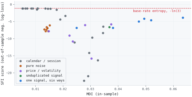
Figure 3. Single-feature scores against in-sample impurity, with the base-rate reference

• Horizontal axis: MDI, so the informative features sit to the right.
• Dashed line: the score an uninformative feature earns, the entropy of the three-class base rate.
• Vertical spread: features pressed against the reference line are the ones a single-feature model cannot separate at all, and they outscore every informative feature.

The best SFI score in the run belongs to tokyo_session, at -1.172, essentially the base-rate value. The six copies of the latent signal score between -6.836 and -3.834. Sorted as though it were an importance column, SFI puts a binary session flag at the top and the actual predictor two thirds of the way down.

The explanation is calibration, not information. A binary session flag splits the data into two blocks and can do nothing else, so the model returns the class balance of each block and is never far from the base rate. A continuous informative feature is different: the forest partitions it finely, finds regions where one class dominates the training data, and predicts those regions with high confidence. Log-loss charges an unbounded penalty for a confident error and a small one for an uncertain miss, so a model that is right more often but occasionally very wrong can score below a model that never commits at all.

SFI is doing what it was designed to do. The value read off it is which features are informative in isolation, and it should be read relative to the base-rate line rather than as a ranking: distance from that line marks the features a one-column model can do something with. Where a probability-scoring metric makes this hard, the metric can be changed. With binary meta-labels the pipeline scores with F1 instead, which counts decisions rather than confidence and does not carry the penalty described above.

Wiring the Analysis into the Training Run

The analysis lives in FeatureEngineeringPipeline, which shares its data loading, triple-barrier labeling and sample-weight search with ModelDevelopmentPipeline and diverges after that. The model pipeline answers which model to deploy. The feature pipeline answers which features are worth computing, and it answers that question against the same labels and weights.

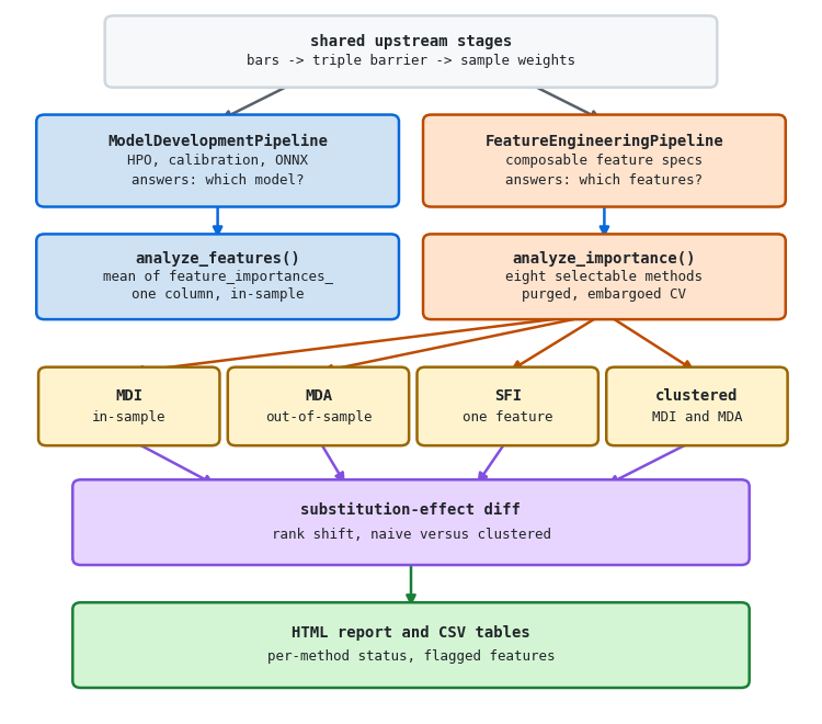
Figure 4. Placement of the feature-importance stage alongside the model training run

• Upper half: both pipelines consume the same bars, triple-barrier events and sample weights, so importances are measured against the labels a model would actually be trained on.
• Left branch: the model pipeline's single in-sample importance column.
• Right branch: the eight selectable methods, the per-cluster diagnostic, and the report they feed.

Features arrive as a list of specifications rather than a fixed set, each one a callable, its parameters, and a name. Any function taking a bar frame and returning a feature frame can be dropped in, and the pipeline records which specification produced which columns so the report can attribute importance back to its source.

pipe = FeatureEngineeringPipeline(
    data_config=data_config,
    feature_configs=[
        {"func": compute_all_microfeatures, "params": {}, "name": "micro"},
        {"func": get_fractal_features,      "params": {}},
        {"func": get_lagged_returns,        "params": {"n_lags": 5}},
    ],
    target_config=target_config,
    label_config=label_config,
    importance_config={
        "methods": ["mdi", "mda", "clustered_mdi", "clustered_mda", "pca"],
        "n_splits": 5,
        "pct_embargo": 0.02,
        "clustering": {
            "dependence_metric": "linear",
            "denoise": True,   # shrink noise eigenvalues before ONC (Part 20)
            "detone": False,  # the leading mode here is the signal, not a market factor
        },
    },
)
importances, catalog, config = pipe.run()

The clustering block is passed straight through to get_feature_clusters, which now accepts denoise, detone, market_components, kde_bwidth and use_effective_sample_size. When denoising is on, the cleaning runs between the correlation matrix and ONC, and the fit diagnostics come back with the partition so the report can state which spectrum produced it. Denoising is defined for a sample correlation matrix, so the call raises rather than proceeding if it is combined with an information-theoretic dependence_metric, and detone without denoise raises for the same reason.

Leaving denoise unset is a supported choice and logs a warning, since a partition built on a raw correlation matrix is the one case where the clustered numbers in this article would not reproduce.

The importance model is not the deployed model. It is a dedicated random forest configured per snippet 8.2, built by the pipeline. That configuration is specific to importance estimation and is not what a deployment model should look like, and a plain forest exposes bare decision trees in estimators_, which MDI reads directly with no unwrapping.

MDA and SFI dominate the runtime, because each fits the model once per fold per feature or per cluster. Neither is in the default method set. On the 44-column matrix used here, MDI took under a second and SFI took roughly fifty.

Reading the Report

Each method runs inside a guard that logs a failure and continues, so one method cannot terminate the run. That guard has a cost worth naming: a method that fails is simply absent from the results, and a report rendering three of eight requested methods is indistinguishable from a report where only three were asked for. The report now opens with a status table listing every requested method, its outcome, and the reason for any failure, before any importance section appears.

The remaining sections are ordered so that the interpretation problems above are visible rather than implicit. Cluster membership is printed in full, because clustered scores are broadcast from it and a partition that merges an informative block into a large one changes every clustered number. SFI is separated from the importance sections and drawn with its base-rate reference line. The dilution table follows the clustered results, so the ratio and the clustered score can be read together.

Alongside the HTML, the pipeline writes:

• one CSV per method,
• a feature catalog mapping each surviving column to its specification and coverage,
• the feature matrix in Parquet format.

All outputs are saved to a versioned artifact directory keyed by symbol, bar type, and date range.

Conclusion

The single averaged importance column a training run produces is not wrong about what the trees did. It is unreliable as a guide to which features to keep, because it divides one predictor's credit among every correlated re-expression of it. On a matrix where the answer was fixed in advance, six copies of one signal summed to eighteen times the best noise column while the weakest copy ranked below eleven features that duplicate nothing.

The correction that recovered the ground truth was clustered MDA, which permutes a whole cluster and leaves no substitute for the model to read. Clustered MDI, run on the identical partition, inverted the ordering, because summing member impurities makes a cluster's score scale with its size. When cluster sizes are unequal, that is a reason to prefer the accuracy variant rather than a reason to distrust clustering.

Two qualifications belong with that conclusion. Every clustered number inherits the partition, and the partition inherits the correlation matrix: on the raw sample correlation one of the six copies clusters with the noise and keeps its diluted score, and only the Part 20 cleaning step recovers it. SFI under log-loss is partly a calibration measurement and is best read against the base-rate line rather than sorted. That makes the partition, and the spectrum behind it, the first thing to inspect in the report rather than the last.

The synthetic market earns its place here because the answer is known in advance, not because the separation is large. A real feature set will not divide this cleanly, and the numbers above should be read as a demonstration that the effect is measurable rather than as an estimate of its size on live data.

Attached Files

File	Location	Description
afml.zip	afml/	The import closure of feature_engineering.py: every module the pipeline needs, with package files and a requirements list. Drop the afml folder onto the import path and the pipeline runs.
feature_engineering.py	afml/production/feature_engineering.py	Feature construction, triple-barrier labeling, sample-weight search, and the importance stage. Adds a per-method status ledger, the per-cluster dilution diagnostic, and the denoising diagnostics carried into the report.
denoising_detoning.py	afml/denoising/denoising_detoning.py	Part 20's module, with clean_corr added: one call from feature panel to cleaned correlation matrix, returning the fit diagnostics. Raises EffectiveSampleSizeError, carrying the correlation matrix and eigendecomposition, when the effective sample size leaves too few observations per variable.
feature_clusters.py	afml/clustering/feature_clusters.py	Clustered feature subsets. get_feature_clusters now cleans the correlation matrix before ONC when denoise is set, and accepts a precomputed matrix so a caller can resume after a failed fit without recomputing it.
importance.py	afml/feature_importance/importance.py	MDI, MDA, clustered variants, and SFI. The MDA permutation now writes back to the frame it scores, and all three methods return float rather than object columns.
feature_engineering_summary.html	reports/	The report produced by the run behind every figure and table in this article: method status, cluster membership, per-method rankings, the SFI section, and the dilution table.