Neural Networks in Trading: The Adaptive Graph Diffusion Model (Attention Module)

Introduction

In the previous article, we were introduced to the SAGDFN framework. We discussed the key principles behind its operation and highlighted its strengths. But the market isn't a museum of architectural models. Here, there is no tolerance for excessive hesitation or lifeless schemes. For a building to stand, it must be built — brick by brick — while checking each level for stability.

The SAGDFN framework was originally conceived as a response to one of the oldest and yet most pressing problems in financial markets: data redundancy and noise that masks true signals. Traditional analysis methods either sank in this flood of information or tried to drain it through crude filtering. SAGDFN, however, offers a different path — not just to filter, but to select intelligently. The framework’s authors proposed retaining only those neighbors that actually influence the system’s behavior. It is similar to an old trading adage: listen to the market, but know how to distinguish the cries of the crowd from the whispers of those who know the way.

The key concept around which the entire architecture is built is Significant Neighbors Sampling, a dynamic system for sampling significant neighbors. Imagine an old port where hundreds of ships arrive every minute, bringing news from all the seas. Not all of them are important to your business: some carry only gossip from foreign markets, while others carry cargo that will lose its value tomorrow. The goal of SAGDFN is to let in only those whose sails truly pull trade in the right direction. To achieve this, the model uses a combination of deterministic importance assessment and controlled randomness — a sort of “wind of change” that prevents the system from becoming stuck in established connections and thereby reduces the risk of overfitting.

Another equally significant element is the α-Entmax mechanism — a mathematical “conductor” of attention distribution. Unlike the gentle yet all-encompassing SoftMax, it does not spread its strength across all inputs, but instead sparsifies the distribution, leaving strong emphasis where it is truly needed. It's similar to an old merchant's wisdom — not to scatter capital on trivial matters, but to invest it in what will yield the greatest return.

SAGDFN is also distinguished by its balance between local and global context. Like an experienced analyst, it can examine the market up close — analyzing adjacent data, individual bars, and local clusters of trades. And at the same time, it keeps the big picture in mind: trends, established patterns, and the structure of long-term flows. In this respect, it acts as a navigator who guides the ship by the stars but does not forget the depth beneath the keel.

The architecture of the SAGDFN framework is modular and extensible, which is particularly valuable in constantly changing trading conditions. There are no stone walls here to confine the researcher. Each block — whether it involves neighbor sampling, attention normalization, or integration with external data sources — can be refined, optimized, or replaced.

The authors’ visualization of the SAGDFN framework is shown below.

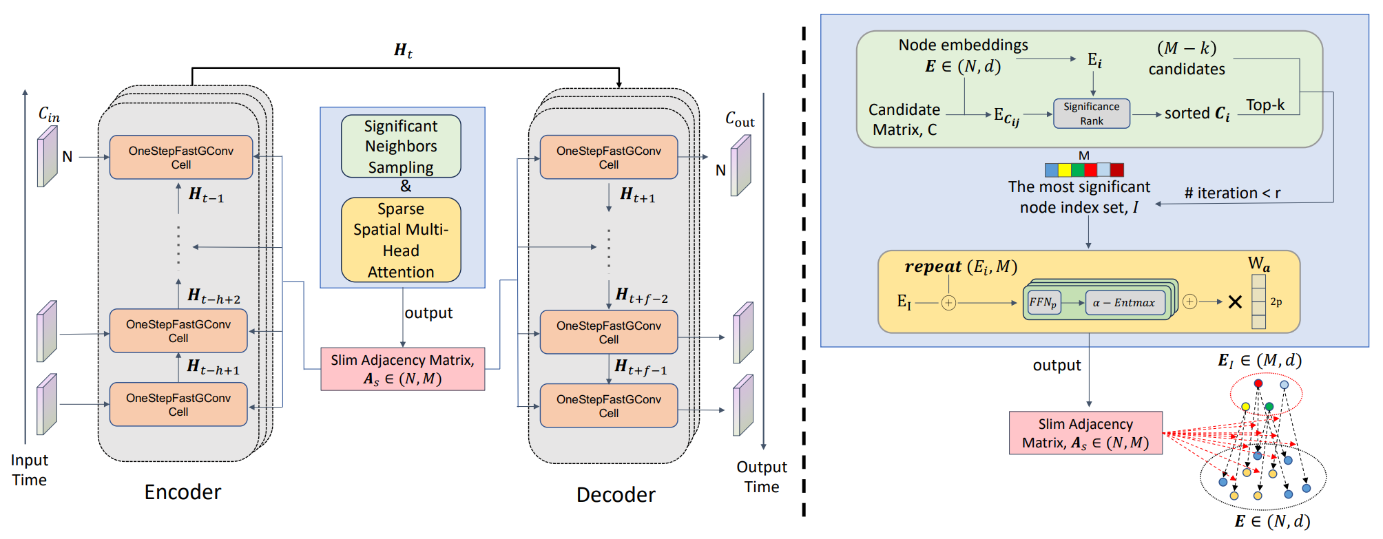
In the practical section of the previous article, we already took the first major step: we implemented the Significant Neighbors Sampling algorithm within the OpenCL context, thereby laying the foundation for the entire structure. We have learned to extract from a massive dataset precisely those connections that truly matter and pass them on to the subsequent computational pipeline without excessive noise. This was not merely a technical experiment, but a crucial stage in the development of a future trading mechanism: without a well-tuned sampling mechanism, it is impossible to build a reliable analysis system.

Today, we continue our work and move on to the next level of integrating our own vision of the approaches proposed by the authors of the SAGDFN framework using MQL5 tools.

Implementation Discussion

After the algorithms of the Significant Neighbors Sampling module — a mechanism for selecting the most significant connections — have been successfully implemented, the next logical step is to move from data preparation to deeper analysis and transformation. Today, we begin by developing the algorithms for the Sparse Spatial Multi-Head Attention module, which will serve as a key tool for extracting structural patterns from the neighbors that have already been selected.

This module acts as a kind of smart sieve, capable not only of processing information but also of directing the model’s attention so that it focuses on truly significant spatial connections without losing sight of the global context. It uses a multi-head attention mechanism, but unlike the classical approach, the framework's authors implement it in a sparse format. This makes it possible to significantly reduce the computational load without compromising the quality of the analysis. Thus, each data stream passes not through a monolithic weight matrix, but through a more efficient yet selectively rich attention network, where each attention head performs its own filtering and highlighting function.

Before proceeding with the actual implementation, it is important to outline our vision of how we will structure our implementation of the algorithms proposed by the framework’s authors and which key points deserve special attention. The framework's creators offer a fairly intuitive and clear approach. To build the graph, they concatenate the embedding of each element pairwise with the embeddings of its nearest neighbors, preselected in the Significant Neighbors Sampling module. Each such pair then passes through a compact fully connected model, which forms the subsequent representation of the edges.

At first glance, the methodology appears transparent and logical, and the processing procedure seems simple and straightforward. However, when this approach is considered in the context of practical implementation — especially on real-world trading data with a high edge density — it becomes clear that this apparent simplicity masks very substantial overhead. Pairwise concatenation of embeddings for each element and its neighbors leads to a significant increase in data volume, which in turn raises the memory requirements. Each pair effectively creates a new vector, and the more such pairs there are, the more resources are required to store them and process them further.

In addition, using a fully connected model for each pair increases the computational load, since each pair must be processed individually. This results in longer execution times and makes the system less flexible when working with large graphs or under conditions of limited computing resources. Thus, despite the visual clarity of this solution, it could become a bottleneck in the process of building an efficient and scalable system.

If we look more closely at the original construct, it becomes clear: the authors use the same small fully connected network to process all pairs [ei ‖ ej], where ei is the embedding of a node and ej is the embedding of one of its selected neighbors. The parameters of this network are common to all pairs: it is not a set of different models, but rather the same set of weights that is reused over and over again. It is precisely this commonality that serves as our lever for acceleration.

A fully connected layer is, by its very nature, a linear transformation combined with nonlinearity. In the linear phase, it multiplies the components of the input vector by the corresponding weights and sums the results. If the input is the concatenation [ei ‖ ej] ∈ R^2d, and the first-layer weight matrix is W ∈ R^{h × 2d}, then the product decomposes into the sum of two terms.

where W1 and W2 ∈ R^{h × d} are the left and right halves of W, respectively.

This simple algebraic observation points the way forward: instead of performing M passes of each ei through the same layer for all of its neighbors, it is more reasonable to compute the projection of each node pi = W1 ei once, and separately compute the neighbor projection ki = W2 ei. In that case, any pair (i,j) at the linear stage is obtained instantly as pi + kj. Then come the same nonlinearity and the next linear attention head, but without repeatedly applying the heavy matrix to the concatenated vector.

In practice, this means that we multiply the initial embedding tensor E by two weight matrices in advance, resulting in two projection tensors. These operations are performed once per batch and vectorize extremely well on the GPU. After that, for each node–neighbor pair, all we have to do is add the corresponding projections. The win is twofold: each ei is multiplied by the query weights W1 exactly once, regardless of how many neighbors it has, and each ej is multiplied by the key weights W2 just once as well, even if it appears in dozens of other lists. The dense part of the work no longer scales with M.

If we focus on asymptotic complexity, the shift in the load profile becomes clear. Naive concatenation requires N * M matrix-vector multiplications of dimension h * 2d, resulting in O(NMhd) for the first linear stage. The refactored path performs two multiplications, EW1 and EW2, in O(Nhd) each, and then only N * M additions of h-dimensional vectors and a lightweight attention head — that is, O(NMh) without the expensive factor d. When d is large and M is not small, the difference is visible right in the profiler output. In terms of memory, the story is similar: instead of storing N * M concatenated vectors of length 2d, we keep two matrix pools, P and K, of size N * h each, and form the sums for the required pairs on the fly. Memory pressure drops, and ALU throughput is used more efficiently.

This same logic fits perfectly with our implementation in MQL5 + OpenCL. To form the projections, we can use a standard convolutional layer with the number of filters equal to 2h, which is run once per pass, regardless of the current set of neighbors. This is important because the list I can change from one iteration to the next, while recomputing the projections still remains stable and inexpensive. Next, for each pair (i,j), we read rows Pi and Kj, sum them element-wise, and apply the attention head. Where there used to be matrix multiplications over concatenated tensors, what remains are clean vector summations and a single small linear layer — operations ideally suited to wide vectorization. If sparse attention normalization is applied on top of this, it operates directly on the resulting logits and does not disrupt the preliminary projection scheme in any way.

There is also a nice bonus when it comes to interpretability. The matrix W1 starts to act as the query projection, while W2 acts as the keys. Their rows and activations show which embedding components more actively shape attention in a specific attention head. In risk management, this is a minor detail that helps explain why the model is focusing on oil rather than bonds at the moment, or why a currency pair has suddenly become the dominant neighbor for tech stocks.

Another important aspect that deserves special attention relates to the use of the α-Entmax function. Its key feature is its ability to smoothly normalize the input data, with the option to adjust the level at which insignificant elements are filtered out. When α==1, this function is equivalent to the standard SoftMax, and when α==2, it approaches Sparse-SoftMax, providing more aggressive zeroing of insignificant values. However, despite the appeal of this idea, it is important to note that the α-Entmax algorithm requires an iterative search for the parameter τ, which inevitably increases the computational complexity and the execution time of the operation. In our implementation, we decided to prioritize efficiency and replaced this function with Sparse-SoftMax. This approach preserves the framework’s design philosophy of excluding insignificant elements from the analysis, while also delivering higher performance and reducing resource consumption during the computation phase.

In the next step, we will carefully integrate this scheme into our existing pipeline. Linear algebra has already done the hard work for us — all that is left is to properly distribute the computations across time and memory so that our multi-head attention optics can focus quickly, precisely, and without unnecessary noise.

Extending an OpenCL Program

Now that we have discussed the architectural principles of the Sparse Spatial Multi-Head Attention module, it is time to put this concept into practice. In the previous step, we emphasized that multiplying the input tensor by the parameter matrix once not only conserves resources but also allows us to preserve all key characteristics of the algorithm, including the selection of the most significant neighbors. In the context of OpenCL, this takes on special significance: here, every operation and every instance of local memory is optimized for high performance.

We start with the SparseMHScores forward pass kernel, which is responsible for computing the weight coefficients between central elements and their most significant neighbors. The kernel is designed so that the processing of each element is as parallel as possible. At the same time, control over the sparsity of the weights is maintained.

__kernel void SparseMHScores(__global const float* data,
                             __global const float* indexes,
                             __global float* scores,
                             const float sparse              ///< [0.0 .. 1.0) sparsity coefficient
                            )
  {
   const int main = (int)get_global_id(0);
   const int slave = (int)get_local_id(1);
   const int head = (int)get_global_id(2);
   const int total_mains = (int)get_global_size(0);
   const int total_slaves = (int)get_local_size(1);
   const int total_heads = (int)get_global_size(2);

First, each global thread obtains the index of its main element main and the local identifier of the neighbor slave. At the same time, the current attention head, head, is determined, which allows all heads to be processed simultaneously and a multidimensional attention map to be created. Next, a local array named Temp is created, which is used to temporarily store intermediate calculations while finding the maximum and minimum values in the block.

   __local float Temp[LOCAL_ARRAY_SIZE];

Next, we retrieve the logit values for the main element and its neighbor from the data arrays. The IsNaNOrInf function ensures that subsequent operations are performed correctly. If the value is invalid (NaN or Inf), it is replaced with 0.

   float value = IsNaNOrInf(data[RCtoFlat(main, head, total_mains, 2 * total_heads, 0)], 0);
   int slave_id = (int)indexes[RCtoFlat(main, slave, total_mains, total_slaves, 0)];
   if(slave_id < total_mains && slave_id >= 0)
      value += IsNaNOrInf(
                  data[RCtoFlat(slave_id, head + total_heads, total_mains, 2 * total_heads, 0)],
                  0);

Please note that we first retrieve the exact neighbor index from the indexes buffer. In this case, special attention is paid to verifying the validity of the obtained index. If a neighbor is out of bounds or has a negative index, it is excluded from the calculations. This ensures the correctness of the calculations and prevents incorrect summation.

Next, the key Sparse-Softmax operation is implemented. First, local maxima and minima are computed using the LocalMax and LocalMin functions, which makes it possible to determine the threshold value. This threshold controls the filtering of insignificant elements: values below the threshold are set to zero, while significant elements pass through an exponential function with normalization by the sum of all elements in the block.

   const float max_value = LocalMax(value, 1, Temp);
   const float min_value = LocalMin(value, 1, Temp);
   const float threshold = (max_value - min_value) * sparse + min_value;
   value = (threshold <= value ? IsNaNOrInf(exp(value - max_value), 0) : 0);
   const float sum = LocalSum(value, 1, Temp);
   value = IsNaNOrInf(value / sum, 0);
//---
   scores[RCtoFlat(slave, head, total_slaves, total_heads, main)] = value;
  }

The result is a sparse but informative weight vector that reflects the importance of each neighbor to the current element. The computed weights are written to the output array scores. The RCtoFlat function converts multidimensional indices into one-dimensional positions. This approach ensures consistent storage of results and allows the next graph convolution stage to use them directly for information aggregation.

Taken together, this kernel implements compact, high-performance, parallel attention processing, ensuring precise weight distribution among elements and their significant neighbors. It preserves the entire logic of the SAGDFN approach proposed by the authors, but makes the computations efficient, scalable, and suitable for practical use on large time series.

Now that we have examined the forward pass in detail and understood how sparse attention weights are formed for each attention head and each element, the next logical step is to implement the backward pass.

The backward pass is necessary for correctly computing gradients during model training. It is responsible for ensuring that errors obtained at the output are accurately propagated back to the embeddings and parameters involved in computing the attention weights. In the context of OpenCL, this means creating a separate kernel that repeats the structure of the forward pass, but focuses on correctly accumulating gradients and accounting for the sparse structure of the weights.

However, there are a few important points worth emphasizing here. First and foremost, the query logit is involved simultaneously in computing all attention coefficients. This means that during the backward pass, it must accumulate the error gradients from all associated information flows, ensuring that error signals are propagated correctly throughout the network.

Second, for neighboring elements, we work with a kind of sparse matrix, which imposes certain constraints and specific considerations on the design of the backward pass algorithm. This structure requires careful consideration of which elements are actually involved in the computations, so that gradients propagate only along active connections, without wasting resources on empty or insignificant positions.

And, of course, we should not forget the specifics of the SoftMax function: changing a single element automatically affects the entire vector, creating interdependence among the coefficients. In our case, for elements that are not among the selected neighbors, we assign a zero weight. At the same time, the error gradient is carefully propagated across the entire attention vector, ensuring that parameters are updated correctly even for those elements that did not actually participate in active connections, thereby preserving the integrity and stability of the backpropagation process.

To gain a more coherent and deeper understanding of how the backward pass kernel works, we should first revisit the logic behind the Sparse Spatial Multi-Head Attention module. During the forward pass, we generated sparse attention scores for selected neighbors using precomputed indices and node projections. These values play a key role in distributing information among the graph nodes, and, consequently, correct propagation of the error in the backward direction is critical for stable model training.

The SparseMHScoresGrad kernel is responsible for carefully distributing the error gradients across each element of the input tensor, taking into account the sparsity and the specifics of SoftMax. In particular, a change in a single logit affects all elements of the attention vector; therefore, even those neighbors that were not included in the final set should receive the proper gradient. This makes it possible to preserve the correct computational structure and avoid disrupting the balance of error distribution.

__kernel void SparseMHScoresGrad(__global float* data_gr,
                                 __global const float* indexes,
                                 __global const float* scores,
                                 __global const float* scores_gr
                                )
  {
   const int main = (int)get_global_id(0);
   const int slave = (int)get_local_id(1);
   const int head = (int)get_global_id(2);
   const int total_mains = (int)get_global_size(0);
   const int total_slaves = (int)get_local_size(1);
   const int total_heads = (int)get_global_size(2);

Each kernel thread is assigned three key indices:

• main — the node for which the gradient is calculated,
• slave — the local index of the neighbor,
• head — attention head.

The Temp buffer in local memory is used to temporarily store intermediate gradient values within a local block of threads, and synchronization via BarrierLoc ensures data consistency during parallel processing.

   __local float Temp[LOCAL_ARRAY_SIZE];
   const uint ls = min((uint)total_slaves, (uint)LOCAL_ARRAY_SIZE);

In the first computation block, the gradients are computed relative to the node being analyzed. First, the attention coefficient for the current neighbor and its index, slave_id, are retrieved.

//--- Calculate gradient by main
     {
      float value = IsNaNOrInf(scores[RCtoFlat(slave, head, total_slaves, total_heads, main)], 0);
      int slave_id = (int)indexes[RCtoFlat(main, slave, total_mains, total_slaves, 0)];
      const float sc_gr = IsNaNOrInf(
                            scores_gr[RCtoFlat(slave, head, total_slaves, total_heads, main)], 0);

The gradient grad is calculated as the difference between the actual weight and the expected value, multiplied by the attention coefficient error gradient sc_gr for the current position.

      float grad = 0;
      for(uint d = 0; d < total_slaves; d += ls)
        {
         if(slave >= d && slave < (d + ls))
            Temp[slave - d] = IsNaNOrInf(sc_gr, 0);
         BarrierLoc;
         for(uint l = 0; l < min(ls, (uint)(total - d)); l++)
            grad += IsNaNOrInf(Temp[l] * ((float)((d + l) == slave && slave_id == main) - value), 0);
         BarrierLoc;
        }

Using local aggregation via Temp followed by summation through LocalSum enables efficient parallel summation, minimizing latency when working with large datasets.

      grad = LocalSum(grad, 1, Temp);
      if(slave == 0)
         data_gr[RCtoFlat(main, head, total_mains, 2 * total_heads, 0)] = grad;
     }

The result is written to the global buffer by only one thread, thereby preventing a race condition.

The second block is responsible for calculating gradients with respect to neighbors. It is important to note here that, hypothetically, every neighbor participates in forming the corresponding attention coefficient (even if it is zero) for each node. Therefore, we treat the value of main as the index of the neighbor being analyzed and iterate through all the nodes.

//--- Calculate gradient by slave
     {
      float grad = 0;
      for(uint d = 0; d < total_mains; d++)
        {
         float value = IsNaNOrInf(scores[RCtoFlat(slave, head, total_slaves, total_heads, d)], 0);
         const float sc_gr = IsNaNOrInf(
                               scores_gr[RCtoFlat(slave, head, total_slaves, total_heads, d)], 0);
         int slave_id = (int)indexes[RCtoFlat(d, slave, total_mains, total_slaves, 0)];

Each thread checks whether the current index corresponds to a neighboring node and carefully adds its contribution to the overall gradient. Local barriers and aggregation via Temp ensure that all threads participate in the process in a coordinated manner.

         float gr = IsNaNOrInf(sc_gr * ((float)(slave_id == d) - value), 0);
         gr = LocalSum(gr, 1, Temp);
         if(slave == 0)
            grad += gr;
        }
      if(slave == 0)
         data_gr[RCtoFlat(main, head + total_heads, total_mains, 2 * total_heads, 0)] =
                                                                             IsNaNOrInf(grad, 0);
     }
  }

The results are stored in the global buffer data_gr for subsequent updates to the model parameters. This approach allows the error to be propagated correctly even in the case of a sparse attention structure, where many elements have a weight of zero, without compromising the integrity of the computations.

It should also be noted that this implementation makes full use of the GPU's parallel processing capabilities. Each thread operates on an independent subset of data, and local memory and barriers minimize conflicts and ensure consistency. This is particularly important when training models on large graphs with thousands of nodes, where traditional sequential gradient computation would be too slow and resource-intensive.

Overall, the SparseMHScoresGrad kernel demonstrates how to efficiently implement backpropagation for sparse multi-head attention, combining accuracy, sparsity preservation, and high computational efficiency.

With that, we can wrap up the implementation phase on the OpenCL program side. The entire process of building a multi-head sparse attention mechanism — from the forward pass with weight computation to the precise distribution of gradients in the backward pass — has been fully migrated to a parallel context. We ensured correct and efficient interaction between nodes and their neighbors, maintained a sparse structure to conserve memory and computational resources, and guaranteed the accuracy of gradients for further model training. The algorithm is now ready to be integrated with the rest of the MQL5 program.

Multi-Head Attention Object

At this stage, we move on to integrating all the components we have developed so far into a single structure within the main program. To do this, we create the CNeuronSNSMHAttention class, which inherits the basic functionality of a convolutional layer from CNeuronConvOCL and combines two key modules: Significant Neighbors Sampling and Sparse Spatial Multi-Head Attention. This class serves as a kind of computational core, bringing together the processes of selecting significant neighbors, forming projections, and calculating attention weights, which ensures a high degree of coherence and consistency in the operation of the entire architecture.

class CNeuronSNSMHAttention   :  public CNeuronConvOCL
  {
   float             fSparse;
   //---
   CNeuronBaseOCL    cNeighbors;
   CNeuronBaseOCL    cRamdomCandidates;
   CNeuronConvOCL    cProjection[2];
   CNeuronBaseOCL    cScores;

   //---
   virtual bool      SignificantNeighborsSampling(CNeuronBaseOCL *NeuronOCL);
   virtual bool      SparseMHScores(void);
   virtual bool      SparseMHScoresGrad(void);
   //---
   virtual bool      feedForward(CNeuronBaseOCL *NeuronOCL) override;
   virtual bool      calcInputGradients(CNeuronBaseOCL *prevLayer) override;
   virtual bool      updateInputWeights(CNeuronBaseOCL *NeuronOCL) override;

public:
                     CNeuronSNSMHAttention(void) {};
                    ~CNeuronSNSMHAttention(void) {};
   //---
   virtual bool      Init(uint numOutputs, uint myIndex, COpenCLMy *open_cl,
                          uint units, uint window, uint heads,
                          uint m_units, float sparse,
                          ENUM_OPTIMIZATION optimization_type, uint batch);
   //---
   virtual int       Type(void)   const   {  return defNeuronSNSMHAttention;   }
   //--- methods for working with files
   virtual bool      Save(int const file_handle) override;
   virtual bool      Load(int const file_handle) override;
   //---
   virtual bool      WeightsUpdate(CNeuronBaseOCL *source, float tau) override;
   virtual void      SetOpenCL(COpenCLMy *obj) override;
  };

The class contains several internal objects, each of which performs a specialized role.

• cNeighbors and cRamdomCandidates are responsible for processing neighbor candidates. The first handles the most significant neighbors, and the second handles random ones, which helps maintain sample diversity and prevents the model from getting locally stuck on narrow data patterns.
• cProjection objects create projections of the initial embeddings into the query and key spaces, which forms the basis for subsequent multi-head attention computations.
• cScores accumulates the calculated attention coefficients, converting them into a sparse influence matrix that will be used during the graph convolution stage.
• The fSparse parameter sets the sparsity coefficient for attention, allowing control over the balance between prediction accuracy and computational load, especially when working with large time series.

At this stage, it is important to note that all internal objects of the CNeuronSNSMHAttention class are declared as static, which allows the class constructor and destructor to remain empty. This design simplifies memory management and makes layer initialization more predictable. The main configuration and deployment of the neural layer architecture are performed through the Init method, which neatly combines all elements and sets their parameters.

bool CNeuronSNSMHAttention::Init(uint numOutputs, uint myIndex, COpenCLMy *open_cl,
                                 uint units, uint window, uint heads,
                                 uint m_units, float sparse,
                                 ENUM_OPTIMIZATION optimization_type, uint batch)
  {
   if(!sparse >= 1 || sparse < 0)
      return false;
   fSparse = sparse;
//---
   if(!CNeuronConvOCL::Init(numOutputs, myIndex, open_cl, heads, heads, 1, units * m_units,
                                                              1, optimization_type, batch))
      return false;

The method's algorithm starts by checking the validity of the sparse sparsity coefficient. If the value is not within the valid range [0, 1), the function immediately returns false, preventing further configuration errors. After that, the fSparse parameter is saved for use in calculating the attention weights.

Next, the parent class is initialized, where the object's basic parameters are set.

It is worth clarifying here that, in this case, we do not limit the functionality of the parent class to merely creating basic interfaces. This is a full-fledged object of our model that performs multi-head attention convolution.

After basic initialization, the step-by-step configuration of internal objects begins. First, the cNeighbors module is initialized; it is responsible for processing the most significant neighbors.

   int index = 0;
   if(!cNeighbors.Init(0, index, OpenCL, units * m_units, optimization, iBatch))
      return false;
   CBufferFloat* temp = cNeighbors.getOutput();
   if(!temp ||
      !temp.Random(0, (float)(units - 1)))
      return false;

At the initial stage, we populate the object's result buffer with random neighbor-index values, ensuring a diverse sample.

A similar sequence is performed for the cRamdomCandidates module, which stores random candidates for expanding the sample.

   index++;
   if(!cRamdomCandidates.Init(0, index, OpenCL, units * m_units, optimization, iBatch))
      return false;
   temp = cRamdomCandidates.getOutput();
   if(!temp ||
      !temp.Random(0, (float)(units - 1)))
      return false;

This approach provides a hybrid neighbor selection mechanism — a combination of significant and random elements.

Next, two objects in the cProjection array are initialized; they form projections of the original embeddings into the query and key spaces. The first object is assigned the SoftPlus activation function, and the second is assigned TANH. This creates a nonlinear transformation and allows the model to account for complex interactions between elements.

   index++;
   if(!cProjection[0].Init(index, 0, OpenCL, window, window, 2 * heads, units, 1,
                                                             optimization, iBatch))
      return false;
   cProjection[0].SetActivationFunction(SoftPlus);
   index++;
   if(!cProjection[1].Init(index, 0, OpenCL, 2 * heads, 2 * heads, 2 * heads, units, 
                                                           1, optimization, iBatch))
      return false;
   cProjection[0].SetActivationFunction(TANH);
   index++;
   if(!cScores.Init(0, index, OpenCL, units * m_units * heads, optimization, iBatch))
      return false;
//---
   return true;
  }

Finally, the cScores object is initialized; it accumulates sparse attention weights and forms the final influence matrix used in graph convolution.

Overall, the Init method is a carefully designed step-by-step initialization process that ensures all components of the layer are configured correctly. It ensures that each object is assigned the necessary dimensions, activation functions, and parameters to operate within a unified architecture. This approach makes the layer flexible and scalable, allowing it to be adapted to various data configurations, different numbers of attention heads, and neighbor sample sizes, while maintaining computational efficiency and high accuracy.

The feedForward method carefully implements the forward pass of data through the module's unified architecture, ensuring sequential interaction among all internal components. First, the SignificantNeighborsSampling method is called, which creates index arrays for significant neighbors. If, for any reason, this step fails, the function immediately returns false, preventing further calculations and preserving the correct state of the layer.

bool CNeuronSNSMHAttention::feedForward(CNeuronBaseOCL *NeuronOCL)
  {
   if(!SignificantNeighborsSampling(NeuronOCL))
      return false;

After the neighbors are successfully selected, a pointer to the NeuronOCL source data object is stored in the local variable inputs, which is then passed through the projection blocks one by one. The loop iterates through each element of the cProjection array. For each element, its own FeedForward method is called; it performs linear and nonlinear transformations on the input tensor, generating query and key projections for the subsequent attention operation.

   CNeuronBaseOCL* inputs = NeuronOCL;
   for(uint i = 0; i < cProjection.Size(); i++)
     {
      if(!cProjection[i].FeedForward(inputs))
         return false;
      inputs = cProjection[i].AsObject();
     }

At the same time, after each block is processed, the input for the next step is reassigned to the output of the previous one, ensuring a continuous data flow and a clean cascaded transformation.

The next step is to call the SparseMHScores method, which computes sparse attention coefficients for all node–neighbor pairs, taking into account the sparsity factor fSparse.

   if(!SparseMHScores())
      return false;
   if(!CNeuronConvOCL::feedForward(cScores.AsObject()))
      return false;
//---
   return true;
  }

The resulting values are accumulated and fed to the convolutional multi-head attention aggregation layer, whose functionality is implemented by the parent class. This is where the final transformation is performed, producing the layer’s final output values.

The entire process is designed to ensure that data flows logically and sequentially through the key stages: first, the selection of significant neighbors; then, the generation of projections; the calculation of sparse attention coefficients; and finally, the aggregation of information. This approach ensures high code readability and makes it easy to integrate additional transformations or optimizations without disrupting the overall architecture. At the end of the method, true is returned, indicating that the forward pass has completed successfully and that the layer is ready for further processing.

The calcInputGradients method is responsible for accurately distributing the error gradient across all internal components of the layer and the input data, ensuring a correct backward pass for training the model. First, it checks whether the pointer to the previous layer, prevLayer, is valid. If it is missing, the function immediately returns false, preventing incorrect calculations.

bool CNeuronSNSMHAttention::calcInputGradients(CNeuronBaseOCL *prevLayer)
  {
   if(!prevLayer)
     return false;

Next, the method of the same name in the parent class is called to distribute gradients at the level of the aggregating layer cScores.

   if(!CNeuronConvOCL::calcInputGradients(cScores.AsObject()))
      return false;
   if(!SparseMHScoresGrad())
      return false;

After that, SparseMHScoresGrad is called, which is responsible for distributing gradients through the sparse attention coefficients generated by the Sparse Spatial Multi-Head Attention module. This is where the characteristics of the sparse neighbor matrix are taken into account, while preserving the architecture’s operating principle.

Next, a loop begins over the cProjection array in reverse order, starting with the last block. For each projection, an input object inputs is defined: if this is not the first block, the output of the previous block is used; otherwise, prevLayer is used.

   int total=(int)cProjection.Size();   
   CNeuronBaseOCL* inputs = NULL;
   for(int i = total-1; i >=0; i--)
     {
      inputs = (i>0 ? cProjection[i-1].AsObject() : prevLayer);
      if(!inputs.CalcHiddenGradients(cProjection[i].AsObject()))
         return false;
     }
//---
   return true;
  }

For each object, the CalcHiddenGradients method is called, which calculates the local gradients of the hidden states, taking into account all accumulated gradients from the next level. This ensures consistent and correct backpropagation through all intermediate layers, while maintaining consistency between the weights and hidden states.

Thus, calcInputGradients performs a complete and structured backward pass through the combined module, accurately distributing gradients across both the sparse attention coefficients and all projection layers, thereby preparing for the subsequent optimization step.

The updateInputWeights method is responsible for sequentially updating the weight parameters of all internal components of the layer after the error gradients have been distributed. It ensures correct model optimization based on the calculated gradients, accurately distributing the changes across each element of the architecture.

bool CNeuronSNSMHAttention::updateInputWeights(CNeuronBaseOCL *NeuronOCL)
  {
   CNeuronBaseOCL* inputs = NeuronOCL;
   for(uint i = 0; i < cProjection.Size(); i++)
     {
      if(!cProjection[i].UpdateInputWeights(inputs))
         return false;
      inputs = cProjection[i].AsObject();
     }

First, the method declares a local pointer to the input data object inputs, which initially points to an external NeuronOCL layer. Next, a loop is started over all cProjection blocks. For each block, the UpdateInputWeights method is called, which applies the calculated gradients to the weight parameters of the current block. If updating the weights fails at any stage, the method immediately returns false, preventing the model from entering an inconsistent state. After the block has been successfully updated, the pointer in inputs is redirected to the output of the current projection so that the next block correctly receives the current input data.

After the loop completes, the method of the same name from the parent class is called; it updates the weights of the multi-head attention aggregation layer, ensuring consistency across all levels of the model. This step is critical for ensuring that the sparse attention coefficients function correctly and for preserving the influence of each selected neighbor in the final prediction function.

   if(!CNeuronConvOCL::updateInputWeights(cScores.AsObject()))
      return false;
//---
   return true;
  }

Finally, the method returns true, indicating that weight optimization was successfully completed for all internal components of the module.

Taken together, the CNeuronSNSMHAttention object makes it possible to neatly combine complex neighbor selection algorithms and multi-head attention within a single structure, ensuring transparency, scalability, and flexibility.

Today's work was intense and productive. We delved deeply into the implementation of the Significant Neighbors Sampling and Sparse Spatial Multi-Head Attention modules. We analyzed their architectural features and examined in detail the mechanisms of forward and backward passes, as well as weight optimization. It is time to take a short break to let the information we have absorbed sink in and lay the groundwork for the next step.

In the next article, we will return to the work we started and carefully bring it to its logical conclusion. We will test the model we have built on historical data, evaluate its robustness and forecast accuracy, and demonstrate the practical applicability of the proposed approach on real financial time series.

Conclusion

In this article, we have taken a detailed look at the practical implementation of the SAGDFN framework's key modules using MQL5 and OpenCL. We analyzed approaches to selecting significant neighbors using Significant Neighbors Sampling, constructing sparse multi-head attention, and efficiently organizing forward and backward passes within a single neural layer. Special attention was paid to optimizing computations: we demonstrated how reusing weight parameters and switching to sparse normalization can significantly reduce memory pressure and speed up data processing.

As a result, the architecture provides both high forecast accuracy and computational efficiency, making the model suitable for handling a large number of time series.

References

• SAGDFN: A Scalable Adaptive Graph Diffusion Forecasting Network for Multivariate Time Series Forecasting
• Other articles in this series

Software used in the article

#	Name	Type	Description
1	Study.mq5	Expert Advisor	Expert Advisor for offline model training
2	StudyOnline.mq5	Expert Advisor	Online model training Expert Advisor
3	Test.mq5	Expert Advisor	Model testing Expert Advisor
4	Trajectory.mqh	Class Library	Structure for describing the system state and model architecture
5	NeuroNet.mqh	Class Library	Class library for building neural networks
6	NeuroNet.cl	Library	Code library for the OpenCL program