

From Option Chain to Risk-Neutral Density: The Market's Own Probability Distribution
 708
 5

Introduction
Two of the previous tools in this options series read the market from the outside in. The implied-volatility surface showed the price of risk, strike by strike and expiry by expiry. The dealer gamma-exposure map showed where hedging flows pin or accelerate price. Both are indispensable, but both stop just short of the question traders care about most: what odds the market assigns to each possible finish level of the underlying. An implied volatility of 22% and a downward skew tell you the market is nervous about the downside, but they do not tell you the probability that the index closes above 5,800 in a month, or the range it expects to stay inside, or how fat the left tail really is. Those are questions about a probability distribution, and the option chain contains that distribution in full. This article extracts it.
The result is called the risk-neutral density. The MQL5 indicator built here reads an option chain (from a CSV file or the broker's native option symbols), fits a smooth volatility smile, applies the Breeden-Litzenberger identity to turn call prices into a density, and draws it on the chart. From it, the tool reads off the probability of finishing above any level, the implied expected move, the implied skew and kurtosis, and a set of confidence bands. It then overlays what the underlying has actually done over the same horizon, so the gap between the two, the risk premium, is there to read.
One honest note up front, because it shapes the design. The density is recovered from option prices and therefore requires an option chain. The realized-return overlay it is compared against is computed from the underlying's ordinary price bars and requires no options. As with the earlier tools, a retail MetaTrader 5 account often carries no option symbols, so the indicator ships with two data paths: a native provider for accounts that do have options, and a CSV provider that runs on any account, fed by a sample chain we generate. Everything the tool computes is only as real as the chain you feed it, and we are explicit about that throughout.
We assume you know options. We will not spend pages defining a call or the smile; we treat those as shared vocabulary and move quickly to how each piece is implemented in MQL5. What we will spend time on is the numerical care the density demands, because the second derivative of a set of noisy quotes is where a naive implementation quietly falls apart.
We will cover:
- What the Risk-Neutral Density Tells Us
- The Black-Scholes Core: Pricing, Inversion, and the Forward
- Why You Cannot Differentiate the Chain Directly
- Reconstructing the Density
- Reading the Distribution
- The Realized Distribution and the Risk Premium
- Two Ways to Feed It: CSV and Native Options
- Drawing the Density on the Chart
- Conclusion
What the Risk-Neutral Density Tells Us
The cleanest way into the idea is a trade you can actually put on. Take three neighbouring call strikes, say 4,950, 5,000 and 5,050, and build a butterfly: buy one 4,950 call, buy one 5,050 call, and sell two 5,000 calls. Draw the payoff at expiry and it is a narrow tent centred on 5,000: it pays a little if the underlying lands right around 5,000, and it pays essentially nothing if the underlying finishes far away in either direction. A butterfly is a bet that says "the underlying finishes near 5,000", and nothing else.
Now ask what that butterfly costs today. Because it only pays off in a narrow band around 5,000, its price is, up to a discount factor, exactly the market's assessed probability that the underlying lands in that band. A cheap butterfly means the market thinks that outcome is unlikely; an expensive one means it thinks it is likely. Slide the butterfly across every strike in the chain, one tent at 4,800, one at 4,900, one at 5,000, one at 5,100, and each price reads off the probability of finishing near that strike. String all of those probabilities together and you have a full distribution: the market's own probability density for the underlying at expiry. A butterfly squeezed this tight is what theory calls an Arrow-Debreu security, a claim that pays off in a single state of the world, so its price simply is the market's probability of that state.

Fig. 1. A tight butterfly pays off only near its centre strike, so its price is the discounted probability of finishing there; sweeping it across strikes traces the whole density
That is the entire idea, and Breeden and Litzenberger (1978) wrote it down as calculus. A tight butterfly is a finite-difference approximation to the second derivative of the call price with respect to strike, so in the limit the density is:
q(K) = e^(rT) * (d^2 C / dK^2)
Here C is the call price as a function of strike K, r is the risk-free rate, T is the time to expiry, and q(K) is the probability density of the underlying at expiry evaluated at price K. The second derivative of the call-price curve, scaled up by the discount factor, is the density. Everything the tool delivers, the probability of finishing above a level, the expected move, the skew and the kurtosis, is a number read off q.
One word in the name earns its keep. This is the risk-neutral density, not the real-world one. It is the distribution implied by option prices, and those prices bake in the premium investors demand for bearing risk, so the density is tilted relative to what the underlying has historically done: heavier on the downside, because crash insurance is expensive. That tilt is not a defect to be corrected; it is the signal. It is what makes this risk-neutral density worth recovering in the first place, rather than assuming the textbook lognormal a naive model would hand you.
The Black-Scholes Core: Pricing, Inversion, and the Forward
Breeden-Litzenberger differentiates call prices, but we never differentiate the raw quotes directly (the next section explains why). Instead we invert each quote to an implied volatility, smooth in that space, and reconstruct clean prices. Both steps rest on the same small Black-Scholes header the earlier tools used, so we keep this section short: the pricer and the inverter are unchanged from the surface and gamma articles, and the only new piece is how we pin down the forward.
The pricer is the textbook Black-Scholes formula for a European option, written to accept a continuous carry (dividend) yield alongside the rate r. It leans on a standard normal CDF (an Abramowitz and Stegun approximation of the error function, accurate to about 1e-7) and its density, both defined just above it in the header. The guard at the top returns pure intrinsic value at or past expiry rather than dividing by zero in the d1 term:
//+------------------------------------------------------------------+
//| Black-Scholes price of a European option.                        |
//|   S     spot price of the underlying                             |
//|   K     strike price                                             |
//|   r     risk-free rate (annual, continuous)                      |
//|   q     dividend / carry yield (annual, continuous)              |
//|   sigma volatility (annual)                                      |
//|   T     time to expiry in years                                  |
//+------------------------------------------------------------------+
double BSPrice(const ENUM_OPT_RIGHT right, const double S, const double K,
               const double r, const double q, const double sigma, const double T)
  {
   if(T <= 0.0 || sigma <= 0.0)
     {
      //--- at/after expiry, value is pure intrinsic
      double intrinsic = (right == OPT_CALL) ? MathMax(S - K, 0.0) : MathMax(K - S, 0.0);
      return(intrinsic);
     }
   double sqrtT  = MathSqrt(T);
   double d1     = (MathLog(S / K) + (r - q + 0.5 * sigma * sigma) * T) / (sigma * sqrtT);
   double d2     = d1 - sigma * sqrtT;
   double disc_r = MathExp(-r * T);
   double disc_q = MathExp(-q * T);
   if(right == OPT_CALL)
      return(S * disc_q * NormCDF(d1) - K * disc_r * NormCDF(d2));
   else
      return(K * disc_r * NormCDF(-d2) - S * disc_q * NormCDF(-d1));
  }
Inverting that pricer for the volatility that reproduces a given quote is a root-find with no closed form. The solver is a hybrid: it keeps a bracket guaranteed to contain the solution, takes a fast Newton step when that step lands inside the bracket, and falls back to bisection whenever Newton misbehaves (vega too small to trust, or a step that would leave the bracket). Deep in- and out-of-the-money quotes, where vega nearly vanishes, are exactly where the plain Newton method flies off, and the bracket is what tames it. A quote below intrinsic value has no valid implied volatility and is flagged with a negative sentinel:
//+------------------------------------------------------------------+
//| Implied volatility by inverting the Black-Scholes price. Uses    |
//| Newton-Raphson (fast) and falls back to bisection whenever a     |
//| Newton step leaves the bracket, which keeps the solver robust for|
//| deep in/out-of-the-money quotes where vega is tiny.              |
//|                                                                  |
//| Returns the implied volatility, or a negative value if no valid  |
//| IV exists for the given inputs (e.g. price below intrinsic).     |
//+------------------------------------------------------------------+
double ImpliedVol(const ENUM_OPT_RIGHT right, const double price, const double S,
                  const double K, const double r, const double q, const double T)
  {
   if(price <= 0.0 || S <= 0.0 || K <= 0.0 || T <= 0.0)
      return(-1.0);

//--- price must sit above intrinsic value or no positive sigma solves it
   double intrinsic = (right == OPT_CALL) ? MathMax(S * MathExp(-q * T) - K * MathExp(-r * T), 0.0)
                      : MathMax(K * MathExp(-r * T) - S * MathExp(-q * T), 0.0);
   if(price < intrinsic - 1e-8)
      return(-1.0);

   double loVol = 1e-4, hiVol = 5.0;   // 0.01% .. 500% brackets the search
   double sigma = 0.2;                 // a sensible starting guess (20%)

   for(int i = 0; i < 100; i++)
     {
      double model = BSPrice(right, S, K, r, q, sigma, T);
      double diff  = model - price;
      if(MathAbs(diff) < 1e-6)
         return(sigma);

      //--- shrink the bracket using the sign of the error (price rises monotonically with sigma)
      if(diff > 0.0)
         hiVol = sigma;
      else
         loVol = sigma;

      double vega = BSVega(S, K, r, q, sigma, T);
      double next;
      if(vega > 1e-8)
         next = sigma - diff / vega;       // Newton step
      else
         next = 0.5 * (loVol + hiVol);     // vega too small: bisect

      //--- if Newton jumped outside the bracket, fall back to bisection
      if(next <= loVol || next >= hiVol)
         next = 0.5 * (loVol + hiVol);

      if(MathAbs(next - sigma) < 1e-8)
         return(next);
      sigma = next;
     }
   return(sigma);
  }
That is the whole of the shared core, and if you have read the earlier articles it is familiar ground. The genuinely new ingredient here is the forward. The density's mean must land on the forward price of the underlying, and we will use that fact as a correctness check, so it matters that the forward is right. We could just compute it from the rate the chain carries, and we do. But the chain also lets us recover the forward a second way, directly from the quotes, through put-call parity. Parity says that at any strike the call minus the put equals the discounted distance from the forward to the strike:
C - P = e^(-rT) * (F - K)
Read as a function of strike, that is a straight line in K: its slope is minus the discount factor, and its intercept is the discount factor times the forward. So we fit a line to the call-minus-put differences by ordinary least squares, across every strike that quotes both a call and a put. That hands us both the discount factor and the forward implied by the market itself, with no assumption about the rate:
//+------------------------------------------------------------------+ //| Recover the forward from put-call parity, independently of the | //| rate carried in the chain. Parity says C - P = DF * (F - K), so | //| a straight line fitted to (C - P) against K across the strikes | //| that quote both rights has slope -DF and intercept DF * F. The | //| forward that falls out is a free consistency check on the mean | //| the density will later report. | //+------------------------------------------------------------------+ void CRiskNeutralDensity::ExtractParityForward(OptionQuote "es[]) { m_parityForward = 0.0; int n = ArraySize(quotes); //--- pair calls and puts on matching strikes for this expiry double xs[], ys[]; for(int i = 0; i < n; i++) { if(quotes[i].expiry != m_expiry || quotes[i].right != OPT_CALL) continue; for(int j = 0; j < n; j++) { if(quotes[j].expiry != m_expiry || quotes[j].right != OPT_PUT) continue; if(MathAbs(quotes[j].strike - quotes[i].strike) > 1e-6) continue; int s = ArraySize(xs); ArrayResize(xs, s + 1); ArrayResize(ys, s + 1); xs[s] = quotes[i].strike; ys[s] = quotes[i].price - quotes[j].price; // C - P break; } } int m = ArraySize(xs); if(m < 2) return; //--- ordinary least squares slope/intercept of (C - P) on K double sx = 0, sy = 0, sxx = 0, sxy = 0; for(int i = 0; i < m; i++) { sx += xs[i]; sy += ys[i]; sxx += xs[i] * xs[i]; sxy += xs[i] * ys[i]; } double denom = m * sxx - sx * sx; if(MathAbs(denom) < 1e-12) return; double slope = (m * sxy - sx * sy) / denom; double intercept = (sy - slope * sx) / m; if(MathAbs(slope) < 1e-12) return; m_parityForward = -intercept / slope; // F = (DF*F) / DF, with DF = -slope }
We keep both forwards: the density is reconstructed against the rate-based forward, and the parity forward becomes an independent second opinion. When the two agree, and later when the density's mean lands on them, we have three separate quantities confirming one another, which is exactly the kind of cross-check that catches a numerical mistake before it reaches the chart.
Why You Cannot Differentiate the Chain Directly
Breeden-Litzenberger is a second derivative, and the obvious implementation is to take it literally: line up the call prices by strike and compute a second difference across each triple of neighbours.
q_i = e^(rT) * (C[i+1] - 2*C[i] + C[i-1]) / (dK^2)
Try it on a real chain and the result is unusable. Differentiating once amplifies whatever noise sits on the quotes; differentiating twice amplifies it again, so the tiny, harmless discrepancies between adjacent mid prices (a penny of bid-ask rounding here, a slightly stale quote there) explode into a jagged curve that swings wildly and dips negative in places. A negative probability density is nonsense, and it is the symptom that tells you the raw second difference has failed. The problem is not Breeden-Litzenberger; it is that the operation is ill-conditioned when applied to noisy prices.

Fig. 2. Left: differencing raw quotes twice yields a spiky, partly-negative curve. Right: smoothing in volatility space first yields a clean density
The fix is the standard one on an options desk, and it is a change of coordinates. Instead of smoothing the prices, we invert every quote to an implied volatility and smooth there. Implied volatility is a slowly varying, well-behaved function of strike (the smile), so a smooth curve through the volatilities is a reasonable, well-conditioned object, whereas a smooth curve through the prices is not. Once we have a smooth smile, we convert it back to a dense set of arbitrage-free call prices through the pricer and differentiate those. The noise never gets to compound, because the prices we differentiate came from a smooth curve, not from the raw quotes.
Before the smile can be splined it has to be built, and there is one choice worth making deliberately: which side of each strike to trust. At a strike below the forward, the put is out-of-the-money and the call is in-the-money; above the forward it is the reverse. The out-of-the-money contract is the liquid, information-bearing one, while its in-the-money mirror is a wider, staler quote that mostly restates intrinsic value. So for each strike we take the out-of-the-money side and fall back to the other only if it is missing. Each survivor becomes one knot of the smile, keyed on log-moneyness rather than raw strike so the fit and its extrapolated tails stay well conditioned:
//+------------------------------------------------------------------+ //| Build the volatility smile the density is differentiated from. | //| For each strike we take the out-of-the-money contract (the put | //| below the forward, the call above it), because those are the | //| liquid, information-bearing quotes; the in-the-money side is its | //| noisy mirror. Each survivor becomes one spline knot, keyed on | //| log-moneyness so the fit and its tails stay well conditioned. | //+------------------------------------------------------------------+ bool CRiskNeutralDensity::BuildSmile(OptionQuote "es[]) { int n = ArraySize(quotes); //--- collect the sorted unique strikes present on this expiry double strikes[]; for(int i = 0; i < n; i++) { if(quotes[i].expiry != m_expiry || quotes[i].iv <= 0.0) continue; if(IndexOf(strikes, quotes[i].strike) < 0) { int s = ArraySize(strikes); ArrayResize(strikes, s + 1); strikes[s] = quotes[i].strike; } } ArraySort(strikes); int nk = ArraySize(strikes); if(nk < 3) { Print("CRiskNeutralDensity: fewer than 3 usable strikes on the chosen expiry"); return(false); } //--- one knot per strike: prefer the out-of-the-money right, fall back to the other ArrayResize(m_knotK, 0); ArrayResize(m_knotIV, 0); for(int k = 0; k < nk; k++) { double K = strikes[k]; ENUM_OPT_RIGHT want = (K < m_forward) ? OPT_PUT : OPT_CALL; double ivWant = -1.0, ivOther = -1.0; for(int i = 0; i < n; i++) { if(quotes[i].expiry != m_expiry || MathAbs(quotes[i].strike - K) > 1e-6) continue; if(quotes[i].iv <= 0.0) continue; if(quotes[i].right == want) ivWant = quotes[i].iv; else ivOther = quotes[i].iv; } double iv = (ivWant > 0.0) ? ivWant : ivOther; if(iv <= 0.0) continue; int s = ArraySize(m_knotK); ArrayResize(m_knotK, s + 1); ArrayResize(m_knotIV, s + 1); m_knotK[s] = K; m_knotIV[s] = iv; } return(ArraySize(m_knotK) >= 3); }
What comes out is a clean set of knots: strike, and the out-of-the-money implied volatility at that strike, sorted and ready to be splined. The density is built off this smile, never off the raw prices, and that single decision is what separates a working tool from the jagged mess of the naive approach.
Reconstructing the Density
With a smile in hand, the reconstruction is a short pipeline: spline the smile, walk a fine grid of strikes, price a call at each one through the smoothed volatility, take the second difference of those prices, and normalise. The class that owns it, CRiskNeutralDensity, exposes a single Build entry point and keeps the grid, the density, and the derived statistics as members; everything the renderer needs is read through const accessors. We take the pipeline in the order the data flows.
The smile is smoothed with a natural cubic spline, implemented directly rather than pulled from a library so the header stays self-contained. The build routine fills the array of second derivatives the evaluator needs; with the natural end conditions (zero curvature at the ends) and fewer than three knots it degrades gracefully to straight lines:
//+------------------------------------------------------------------+
//| Natural cubic spline through (x[i], y[i]) with x ascending. This |
//| fills the second-derivative array the evaluator needs. With the  |
//| natural end conditions (zero curvature at both ends) and fewer   |
//| than three knots the result degenerates to straight lines, which |
//| is exactly what we want as a graceful fallback for a thin smile. |
//+------------------------------------------------------------------+
void SplineBuild(const double &x[], const double &y[], double &y2[])
  {
   int n = ArraySize(x);
   ArrayResize(y2, n);
   if(n < 3)
     {
      ArrayInitialize(y2, 0.0);   // too few knots: fall back to linear
      return;
     }
   double u[];
   ArrayResize(u, n);
   y2[0] = 0.0;
   u[0]  = 0.0;
   for(int i = 1; i < n - 1; i++)
     {
      double sig = (x[i] - x[i - 1]) / (x[i + 1] - x[i - 1]);
      double p   = sig * y2[i - 1] + 2.0;
      y2[i] = (sig - 1.0) / p;
      double d = (y[i + 1] - y[i]) / (x[i + 1] - x[i]) - (y[i] - y[i - 1]) / (x[i] - x[i - 1]);
      u[i] = (6.0 * d / (x[i + 1] - x[i - 1]) - sig * u[i - 1]) / p;
     }
   y2[n - 1] = 0.0;
   for(int k = n - 2; k >= 0; k--)
      y2[k] = y2[k] * y2[k + 1] + u[k];
  }
The evaluator has one subtlety that is worth dwelling on, because getting it wrong puts a phantom spike in the density. Inside the quoted strikes the spline interpolates normally. Beyond the outermost knots, though, we have to extend the smile into strikes the chain never quoted, and the tempting choice, holding the volatility flat, is wrong. Flat extrapolation meets the spline with a different slope, and that slope discontinuity, a kink in the volatility curve, becomes a kink in the reconstructed price, which the second difference reads as a sharp spike and can push negative. The cure is to continue the smile as a straight line at the slope the spline actually reaches at the knot, so the curve is smooth (C1 continuous) across the seam:
//+------------------------------------------------------------------+
//| Evaluate the spline at xq. Beyond the outermost knots the smile  |
//| is continued as a straight line at the slope the spline reaches  |
//| there, rather than snapped flat. Matching that slope keeps the   |
//| curve smooth across the seam (C1); a slope jump there would kink |
//| the reconstructed price and spike its second derivative into a   |
//| phantom negative density. A binary search finds the bracket.     |
//+------------------------------------------------------------------+
double SplineEval(const double &x[], const double &y[], const double &y2[], const double xq)
  {
   int n = ArraySize(x);
   if(n == 0)
      return(0.0);
   if(n < 2)
      return(y[0]);
   if(xq <= x[0])
     {
      //--- linear continuation at the left-end slope of the spline
      double h  = x[1] - x[0];
      double sl = (y[1] - y[0]) / h - h * (2.0 * y2[0] + y2[1]) / 6.0;
      return(y[0] + sl * (xq - x[0]));
     }
   if(xq >= x[n - 1])
     {
      //--- linear continuation at the right-end slope of the spline
      double h  = x[n - 1] - x[n - 2];
      double sr = (y[n - 1] - y[n - 2]) / h + h * (y2[n - 2] + 2.0 * y2[n - 1]) / 6.0;
      return(y[n - 1] + sr * (xq - x[n - 1]));
     }

   int lo = 0, hi = n - 1;
   while(hi - lo > 1)
     {
      int mid = (lo + hi) >> 1;
      if(x[mid] > xq)
         hi = mid;
      else
         lo = mid;
     }
   double hh = x[hi] - x[lo];
   double a  = (x[hi] - xq) / hh;
   double b  = (xq - x[lo]) / hh;
   return(a * y[lo] + b * y[hi] + ((a * a * a - a) * y2[lo] + (b * b * b - b) * y2[hi]) * (hh * hh) / 6.0);
  }
Now the reconstruction itself. We spline the smile in log-moneyness, read the at-the-money-forward volatility to size a grid a few standard deviations wide on each side of the forward, and walk that grid pricing a call at every node. The density is the central second difference of those prices, scaled by the discount factor. Any negative reading is a butterfly-arbitrage artefact, so it is clipped to zero and counted (the count is a data-quality signal we surface later), and the whole thing is normalised to integrate to one:
//+------------------------------------------------------------------+
//| Reconstruct call prices on a fine, uniform strike grid from the  |
//| splined smile, then apply Breeden-Litzenberger. The grid spans a |
//| few at-the-money standard deviations each side of the forward so |
//| the tails are captured; inside the quoted strikes the smile is   |
//| splined, outside it continues linearly. The density is a central |
//| second difference of price in strike, scaled by e^(rT); any      |
//| negative reading is a butterfly-arbitrage artefact and is clipped|
//| to zero and counted. Finally we normalise it to integrate to 1.  |
//+------------------------------------------------------------------+
void CRiskNeutralDensity::BuildDensity(void)
  {
//--- spline the smile in log-moneyness
   double xk[];
   ArrayResize(xk, ArraySize(m_knotK));
   for(int i = 0; i < ArraySize(m_knotK); i++)
      xk[i] = MathLog(m_knotK[i] / m_forward);
   double y2[];
   SplineBuild(xk, m_knotIV, y2);

//--- at-the-money-forward volatility sets the grid width
   m_sigAtm = SplineEval(xk, m_knotIV, y2, 0.0);
   double span = m_tailStds * m_sigAtm * MathSqrt(m_T);
   double kLo  = m_forward * MathExp(-span);
   double kHi  = m_forward * MathExp(span);

   int N = m_gridN;
   ArrayResize(m_gridK, N);
   ArrayResize(m_pdf, N);
   double dK = (kHi - kLo) / (N - 1);

//--- reconstructed call price at each grid strike
   double call[];
   ArrayResize(call, N);
   for(int j = 0; j < N; j++)
     {
      double K = kLo + j * dK;
      m_gridK[j] = K;
      double x  = MathLog(K / m_forward);
      double iv = SplineEval(xk, m_knotIV, y2, x);
      if(iv < 1e-3)
         iv = 1e-3;   // keep the wing volatility strictly positive
      call[j] = BSPrice(OPT_CALL, m_spot, K, m_rate, m_carry, iv, m_T);
     }

//--- Breeden-Litzenberger: density is e^(rT) times the second strike derivative
   double inv_df = 1.0 / m_df;   // e^(rT)
   m_negCount = 0;
   m_negKLo   = 0.0;
   m_negKHi   = 0.0;
   m_pdf[0]     = 0.0;
   m_pdf[N - 1] = 0.0;
   for(int j = 1; j < N - 1; j++)
     {
      double d2 = (call[j + 1] - 2.0 * call[j] + call[j - 1]) / (dK * dK);
      double q  = inv_df * d2;
      if(q < 0.0)
        {
         if(q < -1e-12)
           {
            if(m_negCount == 0 || m_gridK[j] < m_negKLo) m_negKLo = m_gridK[j];
            if(m_negCount == 0 || m_gridK[j] > m_negKHi) m_negKHi = m_gridK[j];
            m_negCount++;
           }
         q = 0.0;   // clip an arbitrage artefact
        }
      m_pdf[j] = q;
     }

//--- normalise to a proper density (trapezoidal integral to 1)
   m_rawIntegral = 0.0;
   for(int j = 0; j < N - 1; j++)
      m_rawIntegral += 0.5 * (m_pdf[j] + m_pdf[j + 1]) * dK;
   if(m_rawIntegral > 0.0)
      for(int j = 0; j < N; j++)
         m_pdf[j] /= m_rawIntegral;

//--- cumulative distribution by running trapezoidal integration
   ArrayResize(m_cdf, N);
   m_cdf[0] = 0.0;
   for(int j = 1; j < N; j++)
      m_cdf[j] = m_cdf[j - 1] + 0.5 * (m_pdf[j] + m_pdf[j - 1]) * dK;
  }
By the end of this routine the object holds three aligned arrays: the strike grid, the density on it, and the cumulative distribution. The raw integral before normalisation is kept as a diagnostic; on a sound chain it comes out within a fraction of a percent of one, and a value far from one is a warning that the smile or the discount factor is off. The grid is uniform in strike, which makes both the second difference and the trapezoidal integrals downstream trivially simple.

Fig. 3. The pipeline: the splined smile becomes a dense set of call prices, whose second difference in strike, scaled by the discount factor, is the density
Reading the Distribution
A density is only useful once you can ask it questions, and every deliverable the tool advertises is a number read off the grid. The moments come first. We integrate the density against strike to get the mean, and against powers of the deviation from the mean to get variance, skewness and kurtosis. The same integration is then repeated in log-return space, because a return skew and kurtosis are what compare like for like against a historical return sample, whereas the price-space moments carry the underlying's scale. The price-space half of the routine is shown here:
//+------------------------------------------------------------------+
//| Compute the moments the density exists to deliver. The mean,     |
//| variance, skewness and kurtosis of the terminal price come from  |
//| trapezoidal integration against the density; the same is done in |
//| log-return space, because it is the return skew and kurtosis     |
//| that compare like for like against a historical return sample.   |
//+------------------------------------------------------------------+
void CRiskNeutralDensity::ComputeStats(void)
  {
   int N = ArraySize(m_gridK);
   if(N < 3)
      return;
   double dK = m_gridK[1] - m_gridK[0];

//--- price-space moments
   double m1 = 0, m2 = 0, m3 = 0, m4 = 0;
   for(int j = 0; j < N - 1; j++)
     {
      double k0 = m_gridK[j],     p0 = m_pdf[j];
      double k1 = m_gridK[j + 1], p1 = m_pdf[j + 1];
      m1 += 0.5 * (k0 * p0 + k1 * p1) * dK;
     }
   m_mean = m1;
   for(int j = 0; j < N - 1; j++)
     {
      double d0 = m_gridK[j]     - m_mean, p0 = m_pdf[j];
      double d1 = m_gridK[j + 1] - m_mean, p1 = m_pdf[j + 1];
      m2 += 0.5 * (d0 * d0 * p0 + d1 * d1 * p1) * dK;
      m3 += 0.5 * (d0 * d0 * d0 * p0 + d1 * d1 * d1 * p1) * dK;
      m4 += 0.5 * (d0 * d0 * d0 * d0 * p0 + d1 * d1 * d1 * d1 * p1) * dK;
     }
   m_std  = MathSqrt(MathMax(m2, 0.0));
   double s3 = m_std * m_std * m_std;
   double s4 = s3 * m_std;
   m_skew = (s3 > 0.0) ? m3 / s3 : 0.0;
   m_kurt = (s4 > 0.0) ? m4 / s4 : 0.0;
The log-return moments that complete ComputeStats are the same integration carried out on ln(K/spot) instead of on K, and they feed the implied-versus-realized skew and kurtosis comparison further on; the full routine is in the attached RndCore.mqh.
The mean is where the tool earns its trust. Under the risk-neutral measure the expected terminal price is exactly the forward, so the mean we integrate out of the density must land on the forward we computed two independent ways in Section 2. When we run the tool on the sample chain, the build routine reports the summary below, and the three numbers line up:
| Reported quantity | Value |
|---|---|
| Expiry (time to expiry, years) | 2026.09.18 (0.1341) |
| Forward, from the rate | 5030.26 |
| Forward, from put-call parity | 5030.30 |
| Density mean, E[S_T] | 5030.81 |
| Implied one-sigma move (price std) | 372.20 (7.4% of spot) |
| Implied return skew | -0.626 |
| Implied return kurtosis | 3.983 |
| Density integral, before normalising | 0.99973 |
| Grid cells clipped for negative density | 0 |
The rate-based forward (5030.26), the parity forward (5030.30) and the density's mean (5030.81) agree to about one part in ten thousand, the integral is within three parts in ten thousand of one, and not a single grid point was clipped for a negative density. That is the evidence that the reconstruction is sound: not that the curve looks nice, but that three independently computed quantities converge on the same number. If the smile were mis-fitted or the discount factor wrong, the mean would drift off the forward and the integral off one, and the discrepancy would be visible here immediately.
The tail probabilities and confidence bands are read off the cumulative distribution. The probability of finishing above a level is one minus the CDF at that level, interpolated between the two grid nodes that straddle it:
//+------------------------------------------------------------------+
//| Probability the underlying finishes strictly above a price. It   |
//| is one minus the CDF, read off the grid with linear interpolation|
//| between the two straddling nodes and clamped outside the grid.   |
//+------------------------------------------------------------------+
double CRiskNeutralDensity::ProbAbove(const double level) const
  {
   int N = ArraySize(m_gridK);
   if(N < 2)
      return(0.0);
   if(level <= m_gridK[0])
      return(1.0);
   if(level >= m_gridK[N - 1])
      return(0.0);
   int lo = 0, hi = N - 1;
   while(hi - lo > 1)
     {
      int mid = (lo + hi) >> 1;
      if(m_gridK[mid] > level)
         hi = mid;
      else
         lo = mid;
     }
   double w   = (level - m_gridK[lo]) / (m_gridK[hi] - m_gridK[lo]);
   double cdf = m_cdf[lo] + w * (m_cdf[hi] - m_cdf[lo]);
   return(1.0 - cdf);
  }
The inverse question, the price at which the cumulative probability first reaches some level, gives the confidence bands: the fifth and ninety-fifth percentiles of where the market thinks price will land, for instance, are just Quantile(0.05) and Quantile(0.95):
//+------------------------------------------------------------------+
//| Inverse CDF: the price at which the cumulative probability first |
//| reaches p. Used for implied confidence bands (e.g. the 5th and   |
//| 95th percentiles of where the market thinks price will land).    |
//+------------------------------------------------------------------+
double CRiskNeutralDensity::Quantile(const double p) const
  {
   int N = ArraySize(m_gridK);
   if(N < 2)
      return(0.0);
   if(p <= 0.0)
      return(m_gridK[0]);
   if(p >= 1.0)
      return(m_gridK[N - 1]);
   for(int j = 1; j < N; j++)
     {
      if(m_cdf[j] >= p)
        {
         double w = (p - m_cdf[j - 1]) / (m_cdf[j] - m_cdf[j - 1]);
         return(m_gridK[j - 1] + w * (m_gridK[j] - m_gridK[j - 1]));
        }
     }
   return(m_gridK[N - 1]);
  }
The implied expected move is simply the price-space standard deviation, exposed as a percentage of spot. On the sample chain that is about 7.4%, meaning the option market is pricing a one-standard-deviation swing of roughly that size over the horizon. Everything a trader reads off the panel, the odds above a level, the expected move, the percentile band, the skew, comes from these few accessors.
The Realized Distribution and the Risk Premium
The risk-neutral density is what the option market prices. To judge it we need what the underlying has actually done, and that comes from a completely separate source: the underlying's own price bars, no options involved. The class CHistoricalDensity samples horizon-length log returns from a close series, takes their moments, and smooths them into a curve we can draw beside the risk-neutral one.
The moments use the population form (dividing by the sample size) rather than the sample form, so that they line up with the density-integral moments on the risk-neutral side, which are population moments by construction. Comparing a population skew against a sample skew would introduce a small, avoidable inconsistency:
//+------------------------------------------------------------------+
//| Population mean, standard deviation, skewness and (raw) kurtosis |
//| of the stored return sample. Population form (divide by n) is    |
//| used so these line up with the density-integral moments on the   |
//| risk-neutral side, which are population moments by construction. |
//+------------------------------------------------------------------+
void CHistoricalDensity::ComputeMoments(void)
  {
   int n = ArraySize(m_ret);
   m_mean = 0;
   m_std  = 0;
   m_skew = 0;
   m_kurt = 0;
   if(n < 2)
      return;

   double s = 0;
   for(int i = 0; i < n; i++)
      s += m_ret[i];
   m_mean = s / n;

   double m2 = 0, m3 = 0, m4 = 0;
   for(int i = 0; i < n; i++)
     {
      double d = m_ret[i] - m_mean;
      m2 += d * d;
      m3 += d * d * d;
      m4 += d * d * d * d;
     }
   m2 /= n;
   m3 /= n;
   m4 /= n;
   m_std = MathSqrt(MathMax(m2, 0.0));
   double s3 = m_std * m_std * m_std;
   double s4 = s3 * m_std;
   m_skew = (s3 > 0.0) ? m3 / s3 : 0.0;
   m_kurt = (s4 > 0.0) ? m4 / s4 : 0.0;
  }
The smooth curve is a Gaussian kernel density estimate: each sampled return contributes a small Gaussian bump, and the density at any point is the average of all those bumps. The bandwidth, which sets how wide each bump is, comes from Silverman's rule of thumb, a sensible default for a roughly bell-shaped sample that needs no tuning:
//+------------------------------------------------------------------+
//| Kernel density at one return: the averaged Gaussian bumps, one   |
//| centred on each sampled return and scaled by the bandwidth.      |
//+------------------------------------------------------------------+
double CHistoricalDensity::DensityAt(const double r) const
  {
   int n = ArraySize(m_ret);
   if(n < 1 || m_bandwidth <= 0.0)
      return(0.0);
   double acc = 0.0;
   double inv = 1.0 / m_bandwidth;
   for(int i = 0; i < n; i++)
     {
      double z = (r - m_ret[i]) * inv;
      acc += 0.3989422804014327 * MathExp(-0.5 * z * z);   // 1/sqrt(2pi) * e^(-z^2/2)
     }
   return(acc * inv / n);
  }
Feeding it is a matter of choosing the horizon so the two distributions describe the same holding period. The build routine takes a chronological close series and forms overlapping log returns over horizon bars, where the horizon is chosen (by the indicator) to match the option's time to expiry in bars:
//+------------------------------------------------------------------+
//| Build from a chronological close series by taking overlapping    |
//| horizon-bar log returns, ln(close[i+horizon] / close[i]). The    |
//| horizon should match the option expiry in bars so the historical |
//| and risk-neutral distributions describe the same holding period. |
//+------------------------------------------------------------------+
bool CHistoricalDensity::FromCloses(const double &close[], const int horizon, const int gridN)
  {
   int n = ArraySize(close);
   if(horizon < 1 || n <= horizon)
     {
      Print("CHistoricalDensity: not enough closes for the requested horizon");
      return(false);
     }
   double ret[];
   ArrayResize(ret, n - horizon);
   int m = 0;
   for(int i = 0; i + horizon < n; i++)
     {
      if(close[i] <= 0.0 || close[i + horizon] <= 0.0)
         continue;
      ret[m++] = MathLog(close[i + horizon] / close[i]);
     }
   ArrayResize(ret, m);
   return(FromReturns(ret, gridN));
  }
Those windows overlap, so each bar feeds several returns and the samples are not strictly independent. That is a deliberate trade: it wrings the most out of a finite history, and since the overlay only needs the shape of the return distribution, the mild autocorrelation is harmless, though it means the far-tail counts are best read as indicative rather than exact.
Now the two curves can be drawn together, and their difference is the whole point. The risk-neutral density is typically wider and more skewed to the downside than the realized one: wider because implied volatility tends to sit above realized volatility (the variance risk premium), and more left-skewed because the demand for crash protection bids up out-of-the-money puts (the crash premium). Where the risk-neutral curve bulges out past the realized one on the downside, the market is charging more for downside protection than history alone would justify, and that gap is a tradeable quantity, not a modelling error.

Fig. 4. The risk-neutral density (what the market prices) against the realized-return distribution (what the underlying actually did over the same horizon)
Two Ways to Feed It: CSV and Native Options
The density does not care where its quotes come from. That is the purpose of the OptionQuote struct: it is a common currency, and anything that can produce an array of them can feed the tool. Unlike the gamma map, the density needs no open interest, only the price at each strike, so the struct is lean:
//+------------------------------------------------------------------+
//| One raw option quote, before the risk-neutral density is built.  |
//| The density is read out of call prices across strikes, so unlike |
//| the gamma-exposure map this struct needs no open interest: only  |
//| the price at each strike carries information. The iv field is    |
//| filled by the provider (inverted from the price, or read from    |
//| the server) so the smile can be smoothed before differentiating. |
//+------------------------------------------------------------------+
struct OptionQuote
  {
   ENUM_OPT_RIGHT    right;
   double            strike;
   datetime          expiry;
   double            price;     // market mid price
   double            spot;      // underlying price
   double            rate;      // risk-free rate
   double            iv;        // filled in by the provider (-1 if invalid)
  };
The CSV provider reads a chain file from the terminal's MQL5\Files sandbox and runs on any account, which is what makes the tool reproducible by everyone. It expects the column order right, strike, expiry, mid, spot, rate, and because it splits each line itself and reads only the first six fields, a chain that carries a trailing open-interest column (the gamma-map format) loads here unchanged. The implied volatility is inverted as each row is read:
//+------------------------------------------------------------------+
//| Parse the CSV chain into a flat quote list. Each non-empty line  |
//| after the header is split on commas; a row with fewer than six   |
//| fields, or a non-positive strike, is skipped rather than trusted.|
//+------------------------------------------------------------------+
bool CRndProviderCSV::Load(const string filename, OptionQuote &out[])
  {
   int h = FileOpen(filename, FILE_READ | FILE_TXT | FILE_ANSI);
   if(h == INVALID_HANDLE)
     {
      PrintFormat("CRndProviderCSV: cannot open %s (err %d)", filename, GetLastError());
      return(false);
     }
   ArrayResize(out, 0);

   datetime now = TimeCurrent();
   if(now == 0)
      now = TimeLocal();

   bool header = true;
   while(!FileIsEnding(h))
     {
      string line = FileReadString(h);
      StringTrimLeft(line);
      StringTrimRight(line);
      if(StringLen(line) == 0)
         continue;
      if(header)
        {
         header = false;   // the first non-empty line is the column titles
         continue;
        }

      string f[];
      int nf = StringSplit(line, (ushort)',', f);
      if(nf < 6)
         continue;         // not enough columns to be a usable quote
      for(int c = 0; c < nf; c++)
         StringTrimRight(f[c]);

      OptionQuote q;
      string rr = f[0];
      StringToUpper(rr);
      q.right  = (StringFind(rr, "P") >= 0) ? OPT_PUT : OPT_CALL;
      q.strike = StringToDouble(f[1]);
      q.expiry = StringToTime(f[2]);
      q.price  = StringToDouble(f[3]);
      q.spot   = StringToDouble(f[4]);
      q.rate   = StringToDouble(f[5]);
      if(q.strike <= 0.0)
         continue;

      double T = (double)(q.expiry - now) / (365.0 * 24 * 3600);
      q.iv = ImpliedVol(q.right, q.price, q.spot, q.strike, q.rate, 0.0, T);

      int s = ArraySize(out);
      ArrayResize(out, s + 1);
      out[s] = q;
     }
   FileClose(h);
   PrintFormat("CRndProviderCSV: loaded %d rows from %s", ArraySize(out), filename);
   return(ArraySize(out) > 0);
  }
The sample chain shipped with the project is a synthetic index at 5,000 with an equity-style skew (out-of-the-money puts carrying higher volatility than out-of-the-money calls) across two expiries. Its first rows look like this:
| right | strike | expiry | mid | spot | rate |
|---|---|---|---|---|---|
| C | 3600.00 | 2026.09.18 | 1421.9688 | 5000.00 | 0.0450 |
| P | 3600.00 | 2026.09.18 | 0.2864 | 5000.00 | 0.0450 |
| C | 5000.00 | 2026.09.18 | 162.3541 | 5000.00 | 0.0450 |
| P | 5000.00 | 2026.09.18 | 132.2397 | 5000.00 | 0.0450 |
The native provider is the path an options-enabled account uses day to day: point it at an underlying and it builds the chain from the broker's live option symbols. It enumerates every symbol, keeps the options whose SYMBOL_BASIS matches the requested underlying, and reads the strike, expiry, right and mid price from each. It prefers the server's own implied volatility when the server publishes one, and inverts the mid price otherwise; both rights are kept because the smile build selects the out-of-the-money side per strike:
//+------------------------------------------------------------------+
//| Enumerate all symbols, collect the options on the requested      |
//| underlying, and build one OptionQuote per contract. The mid      |
//| price comes from the current bid/ask; the implied volatility is  |
//| the server's own when it publishes one, otherwise it is inverted |
//| from the price. Both rights are kept: the density build selects  |
//| the out-of-the-money side per strike and needs both available.   |
//+------------------------------------------------------------------+
bool CRndProviderNative::Load(const string underlying, const double rate, OptionQuote &out[])
  {
   ArrayResize(out, 0);
   int total = SymbolsTotal(false);      // false = all symbols, not just Market Watch
   if(total <= 0)
     {
      Print("CRndProviderNative: no symbols available");
      return(false);
     }

   double spot = SymbolInfoDouble(underlying, SYMBOL_BID);
   if(spot <= 0.0)
      spot = SymbolInfoDouble(underlying, SYMBOL_LAST);

   datetime now = TimeCurrent();
   if(now == 0)
      now = TimeLocal();
   int found = 0, withServerIV = 0;

   for(int i = 0; i < total; i++)
     {
      string sym = SymbolName(i, false);
      if(!IsOption(sym))
         continue;

      //--- match the underlying via SYMBOL_BASIS (the derivative's base asset)
      string basis = SymbolInfoString(sym, SYMBOL_BASIS);
      if(basis != underlying)
         continue;

      //--- make sure the symbol's quotes are available
      SymbolSelect(sym, true);

      OptionQuote q;
      long right = (long)SymbolInfoInteger(sym, SYMBOL_OPTION_RIGHT);
      q.right  = (right == SYMBOL_OPTION_RIGHT_PUT) ? OPT_PUT : OPT_CALL;
      q.strike = SymbolInfoDouble(sym, SYMBOL_OPTION_STRIKE);
      q.expiry = (datetime)SymbolInfoInteger(sym, SYMBOL_EXPIRATION_TIME);
      q.spot   = spot;
      q.rate   = rate;

      //--- option mid price from the current bid/ask (fall back to last)
      double bid = SymbolInfoDouble(sym, SYMBOL_BID);
      double ask = SymbolInfoDouble(sym, SYMBOL_ASK);
      q.price = (bid > 0.0 && ask > 0.0) ? 0.5 * (bid + ask) : SymbolInfoDouble(sym, SYMBOL_LAST);

      //--- prefer the server-computed implied volatility if present
      double serverVol = SymbolInfoDouble(sym, SYMBOL_PRICE_VOLATILITY);
      double T = (double)(q.expiry - now) / (365.0 * 24 * 3600);
      if(serverVol > 0.0)
        { q.iv = serverVol / 100.0; withServerIV++; }    // property is a percentage
      else
         q.iv = ImpliedVol(q.right, q.price, q.spot, q.strike, q.rate, 0.0, T);

      int s = ArraySize(out);
      ArrayResize(out, s + 1);
      out[s] = q;
      found++;
     }

   PrintFormat("CRndProviderNative: underlying=%s spot=%.4f  options found=%d  server IV on %d",
               underlying, spot, found, withServerIV);
   if(found == 0)
      Print("CRndProviderNative: no option symbols matched. This account/broker may not offer options, or the underlying name differs from SYMBOL_BASIS. Use the CSV source to demonstrate the tool.");
   return(found > 0);
  }
Both providers end at the same place: an array of OptionQuote with implied volatilities filled in. Hand either one to CRiskNeutralDensity::Build and you get the same density. That interchangeability is what keeps the renderer, and the reader, indifferent to where the numbers came from.
Drawing the Density on the Chart
The indicator, RndProfile.mq5, turns the density into a self-contained panel drawn with MetaTrader's 2D CCanvas layer. There is no 3D and no DirectX here; the density is a curve, and a curve wants a clean flat panel with two axes, the risk-neutral density and the realized overlay on it, the spot and forward marked, and a header carrying the headline numbers. The whole thing is a bitmap the size of the chart, redrawn on a size change and on demand when you press R.
One piece of that panel is worth a warning, because it cost real time. The card behind the plot has to be opaque so the density reads cleanly, while the margin around it stays transparent so the chart shows through, which means the bitmap needs per-pixel alpha. The obvious canvas format for that, COLOR_FORMAT_ARGB_NORMALIZE, renders the "opaque" card as semi-transparent regardless of the alpha you set, and candles bleed through it. Switching to COLOR_FORMAT_ARGB_RAW gives a genuinely opaque card, but RAW does no alpha blending at all, so any translucent fill you wanted has to be pre-mixed as an opaque tone against the card colour. That is why the palette carries explicit muted-cyan and faint-column tones rather than a translucent cyan with a low alpha:
//+------------------------------------------------------------------+
//| Resolve the theme into an opaque ARGB palette once. The bitmap is|
//| drawn in RAW mode so its alpha is not blended by the terminal;   |
//| the card is fully opaque and the "translucent" area and band     |
//| tones are pre-mixed against the card colour instead of relying on|
//| alpha. The card, text, area and spot tones swap with the theme.  |
//+------------------------------------------------------------------+
void ResolvePalette(void)
  {
   g_rndLine  = ColorToARGB(C'46,196,214', 255);    // risk-neutral density line (cyan)
   g_histLine = ColorToARGB(C'240,170,60', 255);    // realized-return density (amber)
   g_fwd      = ColorToARGB(C'150,150,160', 255);   // forward marker
   if(InpTheme == RND_THEME_LIGHT)
     {
      g_panel   = ColorToARGB(clrWhiteSmoke, 255);
      g_grid    = ColorToARGB(clrSilver);
      g_text    = ColorToARGB(clrBlack);
      g_textDim = ColorToARGB(clrDimGray);
      g_rndFill = ColorToARGB(C'150,205,215', 255); // pale cyan area on a light card
      g_band    = ColorToARGB(C'225,227,232', 255); // faint central-interval column
      g_spot    = ColorToARGB(clrBlack);
     }
   else
     {
      g_panel   = ColorToARGB(C'22,24,30', 255);
      g_grid    = ColorToARGB(C'70,74,86');
      g_text    = ColorToARGB(clrWhiteSmoke);
      g_textDim = ColorToARGB(clrSilver);
      g_rndFill = ColorToARGB(C'30,66,78', 255);    // muted cyan area on a dark card
      g_band    = ColorToARGB(C'34,39,50', 255);    // faint central-interval column
      g_spot    = ColorToARGB(clrWhite);
     }
  }
Drawing the density curve then has to fill the area under it without seams. Filling one vertical line per grid node leaves gaps where two nodes round to the same pixel column, so instead we walk the pixel columns of the plot, interpolate the density at each column's price, and draw the fill column by column; the smooth outline is a single anti-aliased polyline over the grid nodes:
//+------------------------------------------------------------------+
//| Draw the risk-neutral density: a solid area under the curve plus |
//| an anti-aliased outline. The area is filled one screen column at |
//| a time from an interpolated density so it stays seamless, and the|
//| outline is drawn over the grid points clipped to the frame.      |
//+------------------------------------------------------------------+
void DrawRndCurve(void)
  {
//--- filled area, one interpolated column at a time (no seams)
   int xa = XOf(g_xMin), xb = XOf(g_xMax);
   for(int x = xa; x <= xb; x++)
     {
      double price = g_xMin + (double)(x - g_plotX0) / (g_plotX1 - g_plotX0) * (g_xMax - g_xMin);
      int y = YOf(PdfAt(price));
      if(y < g_plotY1)
         g_canvas.LineVertical(x, y, g_plotY1, g_rndFill);
     }

//--- smooth outline over the grid points
   int N = g_rnd.NGrid();
   int xs[], ys[];
   ArrayResize(xs, N);
   ArrayResize(ys, N);
   int m = 0;
   for(int i = 0; i < N; i++)
     {
      double K = g_rnd.GridK(i);
      if(K < g_xMin || K > g_xMax)
         continue;
      xs[m] = XOf(K);
      ys[m] = YOf(g_rnd.Pdf(i));
      m++;
     }
   ArrayResize(xs, m);
   ArrayResize(ys, m);
   if(m >= 2)
      g_canvas.PolylineAA(xs, ys, g_rndLine);
  }
The realized curve is drawn the same way, with one conversion: the kernel density is estimated in return space, so each point is mapped to a price through spot times the exponential of the return, and its height is divided by that price to turn a return density into a price density. That division is what lets the two curves share a single vertical scale and integrate to the same total, so their heights are directly comparable. The header assembles the headline numbers, the probability above spot, the expected move, the percentile band, and the implied versus realized skew and kurtosis, and a small legend keys the colours.
Attach the indicator, leave the source on CSV, and the sample chain draws immediately. The density is a clean, left-skewed bell: its peak sits at the forward, just above spot, and its left tail is visibly longer than its right, the crash premium made literal. The header reads off the numbers a trader wants at a glance.
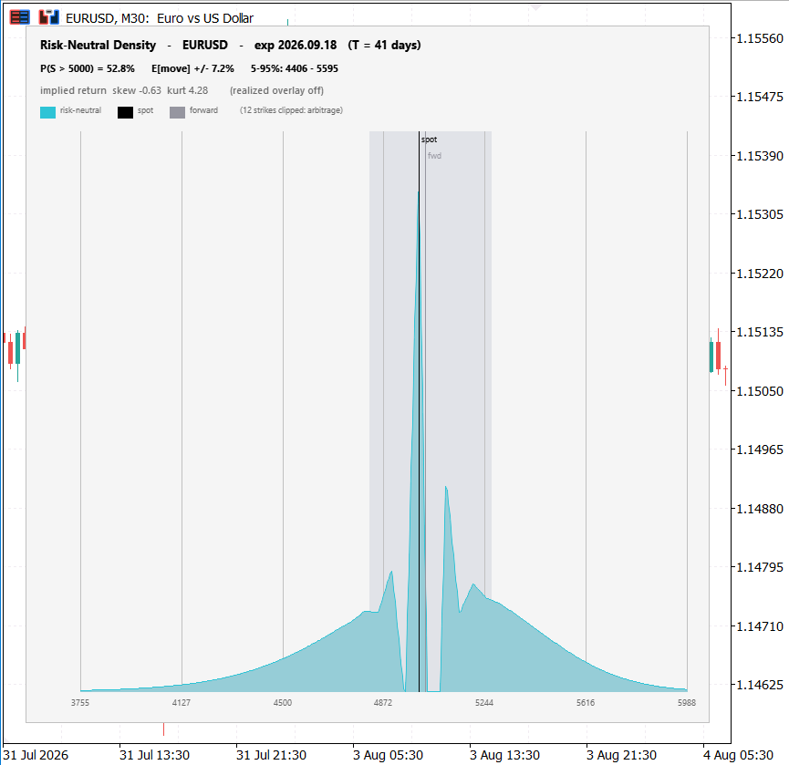
Fig. 5. The RND Profile panel on the sample chain: the density peaks at the forward, the left tail is fatter than the right, and the header carries the probabilities and moments
Turn the realized overlay on, attach the tool to the underlying's own chart so the history matches the chain, and the second curve appears beside the first. Reading the two together is the payoff the tool was built for, and the panel now puts that comparison one glance away.
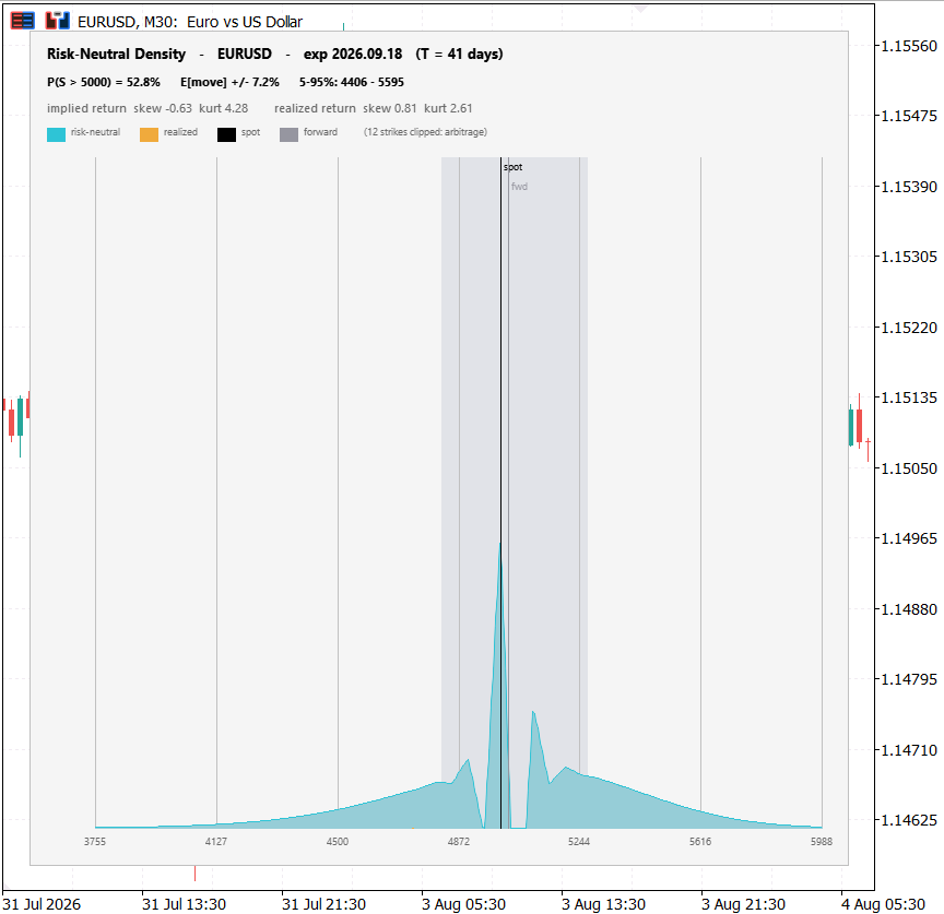
Fig. 6. With the overlay on, the realized-return distribution is drawn beside the risk-neutral one on a shared vertical scale
Conclusion
We set out to recover the one thing the surface and the gamma map leave unsaid: the market's own probability distribution for the underlying at expiry. We got there by treating a butterfly spread as a bet on an outcome, recognising Breeden-Litzenberger as the calculus of that bet, and then doing the numerical work carefully enough that the second derivative of noisy quotes came out as a clean, non-negative density.
- Smooth in volatility space, never in price space. Differentiating raw quotes twice is ill-conditioned; inverting to a smile, splining that, and reconstructing arbitrage-free prices is what makes the density usable.
- Continue the smile smoothly across the seam. Flat extrapolation beyond the outer knots kinks the price curve and spikes the density; continuing at the fitted slope (C1) removes the phantom, and the clipped-negative count drops to zero on a sound chain.
- Let the mean check the work. The density's mean must equal the forward, computed independently from the rate and from put-call parity; three numbers agreeing to one part in ten thousand is the proof the pipeline is right.
- Read the premium, not just the density. Drawn against the realized-return distribution, the risk-neutral density shows where the market charges more for risk than history alone would justify, and that gap is the tradeable signal.
From here the natural extensions are a full term structure of densities (one per expiry, watched over time), and using the implied probabilities directly as a sizing or filter input in an Expert Advisor. Both build on exactly the engine developed here.
Getting the Source Code via MQL5 Algo Forge
All source files are attached to this article below, but the full repository is also available on MQL5 Algo Forge, the community's Git-based platform for sharing and collaborating on trading projects.
| File name | Description |
|---|---|
| MQL5\Include\RND\BlackScholes.mqh | Black-Scholes pricer, vega, and the hybrid Newton/bisection implied-volatility inversion |
| MQL5\Include\RND\RndData.mqh | The OptionQuote struct and the CSV chain provider |
| MQL5\Include\RND\RndCore.mqh | CRiskNeutralDensity: the cubic spline, the density reconstruction, the moments and quantiles |
| MQL5\Include\RND\HistoricalDensity.mqh | CHistoricalDensity: the realized-return moments and Gaussian kernel density estimate |
| MQL5\Include\RND\RndProviderNative.mqh | The native MetaTrader 5 option-symbol chain provider |
| MQL5\Indicators\RND\RndProfile.mq5 | The indicator: the CCanvas panel that draws the density and the realized overlay |
| MQL5\Files\RND\rnd_chain_sample.csv | Sample option chain (synthetic index at 5000, equity-style skew) for the CSV path |
| MQL5\Files\RND\rnd_chain_flatvol.csv | Flat-volatility control chain, whose density is a known lognormal for validation |
Warning: All rights to these materials are reserved by MetaQuotes Ltd. Copying or reprinting of these materials in whole or in part is prohibited.
This article was written by a user of the site and reflects their personal views. MetaQuotes Ltd is not responsible for the accuracy of the information presented, nor for any consequences resulting from the use of the solutions, strategies or recommendations described.

 How to Obtain Synchronized Arrays for Use in Portfolio Trading Algorithms
 Neural Networks in Trading: Heterogeneity-Informed Meta-Parameter Learning (Key Components)
 Neural Networks in Trading: Heterogeneity-Informed Meta-Parameter Learning (Conclusion)
 Building a News Filter Engine in MQL5 Using a Local Economic Calendar File

- Free trading apps
- Over 8,000 signals for copying
- Economic news for exploring financial markets
You agree to website policy and terms of use
Animated images are evil (inconvenient, hard to percept, the animation itself does not add any value - all of these applies specifically to the article animations, not to animations in general, when they make sense). Why not to publish every image as a static one with the whole information freezed at the last frame?
Never heard someone call animated images evil, but I get your point. A GIF cannot be paused, rewound or zoomed, so if you miss a step you are waiting for the loop to come round again.
Where I would push back is the idea that the motion never carries anything. In the butterfly figure the point is the sweep across strikes, and in the pipeline figure it is the order the stages happen in. A single frame shows the result but not the sequence, and the sequence was the thing I was trying to teach.
That said, some animations are cumulative so the final frame does hold the full picture, and publishing a static version of it instead of the sequence is a better option. Thanks for the advice.
Where I would push back is the idea that the motion never carries anything. In the butterfly figure the point is the sweep across strikes, and in the pipeline figure it is the order the stages happen in. A single frame shows the result but not the sequence, and the sequence was the thing I was trying to teach.
Another thing that is not clear for me, why you call the distibution of the butterfly prices densities and require them to behave like probabilities, that's being positive. Actually, buying 2 sideways strikes and selling the center you got a positive (conditional) outcome at the center and negatives everywhere around (your picture does not show this, BTW). BSM provides you with a theoretic price of one specific option, not a butterfly - how can you compare them?
A butterfly doesn't need its own model, it's:
C(K-h) - 2C(K) + C(K+h)So any price function values it by arithmetic. BSM here is only the map between price and implied volatility, not a distributional assumption: every strike is priced at its own vol off the fitted smile. A single vol would give back a lognormal by construction, which is why it isn't done that way. The smile is what makes the curve non-lognormal, and its curvature is the signal.