

Building Volatility Models in MQL5 (Part V): Implementing EGARCH as an Alternate Asymmetric Volatility Process
 859
859
 0
0

Contents
- Introduction
- GARCH's Positivity Constraints: The Problem
- Exponential GARCH: The Solution
- EGARCH MQL5 Implementation
- Tests for Estimating Leverage Effects
- EGARCH Indicators
- Conclusion
Introduction
Consider this scenario: you fit a conditional volatility model after running diagnostics (ACF and PACF) and selecting a reasonable hyperparameter set. The optimization converges, but one volatility parameter has a p-value of 0.99999 (effectively 1), indicating it is statistically insignificant. Upon inspecting the parameter itself, you find it is nearly zero, suggesting something is wrong. Should you try a different model configuration, or is the issue elsewhere?
Standard GARCH-like models face a limitation due to the requirement that predicted conditional variance must remain positive. This necessity forces non-negative boundaries on the model's parameters, which can restrict their ability to capture complex dynamics. In 1991, economist Daniel Nelson introduced the Exponential GARCH (EGARCH) model to address this issue while also enabling the modeling of leverage effects. This article implements EGARCH in MQL5. It first illustrates the positivity-constraint limitation of standard GARCH on real data, then details EGARCH and its MQL5 implementation. It also presents tests for leverage effects and concludes with several EGARCH-based indicators.
GARCH's Positivity Constraints: The Problem
In a standard GARCH model—specifically the foundational GARCH(1,1)—the conditional variance is calculated as a linear combination of past squared residuals and past variances. Because this equation relies on raw variance, the model requires strictly positive values; negative variance is mathematically impossible. To prevent the conditional variance from dropping below zero, econometricians must impose strict constraints during estimation: omega > 0, alpha >= 0, and beta >= 0.
If a maximum likelihood estimation algorithm attempts to fit the data by pushing a parameter into negative territory, the model breaks. The constraints prevent this, forcing the optimization algorithm to settle on parameter values that adhere to the boundaries rather than accurately reflecting the dataset. The script GARCH_ParameterPositivityLimitation.mq5 demonstrates how such a scenario can manifest. It configures a standard GARCH model, fits it to a specific sample of returns, and displays the resulting parameters and p-values in the (MetaTrader 5) terminal's journal tab.
//--- --- Step 5: Model Initialization ---
//--- Instantiate the continuous tracking constant mean container wrapper
   ZeroMean garch_model;
//--- Pass structural parameters down into the optimization initialization routine
   if(!garch_model.initialize(garch_spec))
      return;
//--- --- Step 6: Parameter Optimization (Fitting) ---
//--- Trigger the non-linear execution optimizer loop (SLSQP engine solver)
   ArchModelResult garch_params = garch_model.fit();
//--- --- Step 7: Optimization Convergence Guard ---
//--- Verify that the resulting parameters array size matches the model criteria configurations
   if(!garch_params.params.Size())
     {
      Print("Convergence failed ", GetLastError());
      return;
     }
//--- --- Step 8: Results Output Extraction ---
//--- Print optimal target parameter solutions to the MetaTrader Terminal panel
   Print("GARCH model parameters");

//--- Extract statistical asymptotic standard deviation errors mapped out to individual p-values
   vector pv = garch_params.pvalues();
   Print("Check GARCH model pvalues.\nA corresponding pvalue of 1 or 0.99 is an indication of a"
         "\n parameter being limited  by a boundary constraint."
         "\n Meaning the model parameters are not a reflection of the observed data:");
//--- Get the volatility parameter names
//--- Notice that the full model is anchored by a ZeroMean mean model
   string pnames = garch_model.volatility().parameterNames();
   string vol_parameter_labels[];
//--- Organize parameter names into array for display
   int labels = StringSplit(pnames,StringGetCharacter(",",0),vol_parameter_labels);
//--- Check number of labels is equal to number of model parameters
   if(labels != int(pv.Size()))
      return;
//--- Display pvalues
   PrintFormat("%10s %10s %10s","Name","Value","Pvalue");
   for(ulong i = 0; i < pv.Size(); ++i)
     {
      //--- Log individual calculated p-values step-by-step to evaluate structural significance
      PrintFormat("%10s %10.8f %10.8f",vol_parameter_labels[i], garch_params.params[i], pv[i]);
     }
Running the script with default parameters produces the following output.
GARCH model parameters
Check GARCH model pvalues.
A corresponding pvalue of 1 or 0.99 is an indication of a
parameter being limited  by a boundary constraint.
Meaning the model parameters are not a reflection of the observed data:
Name      Value     Pvalue
omega    0.05541409 0.41632390
alpha[1] 0.00012291 0.99724737
beta[1]  0.69987709 0.02815346
Here, we observe that one parameter's p-value is very close to 1, while the corresponding parameter value is nearly zero. This occurs because the optimizer likely attempted to move the search below zero but was restricted by the constraints. Consequently, it settled on a near-boundary value that yields the highest possible log-likelihood under those restrictions. The result is a set of model parameters that do not accurately describe the observed data. The corresponding p-values highlight this phenomenon. The model's parameters cannot be allowed to take on negative values due to the constraints. Simultaneously, those same constraints are limiting the parameter search. This is the dilemma.
Exponential GARCH: The Solution
Exponential GARCH (EGARCH) is a time-series econometric model developed to address the limitations of Robert Engle's original Autoregressive Conditional Heteroskedasticity (ARCH) framework and Tim Bollerslev's Generalized Extension (GARCH). Introduced in the academic paper "Conditional Heteroskedasticity in Asset Returns: A New Approach," Daniel Nelson designed EGARCH primarily to capture the leverage effect. By modeling the natural logarithm of conditional variance rather than the raw variance itself, Nelson ensured that predicted volatility remained positive without imposing non-negativity constraints on the model's parameters during estimation. The leverage effect, representing asymmetry in volatility, has been covered extensively in a previous article.

Omega represents the constant baseline or intercept of the model. Because the model predicts the log of variance, omega dictates the longer-term, scale-adjusted anchor of the process. If all recent shocks are stripped away, omega determines the starting level of the asset's log-volatility. A positive value implies that the baseline log-variance is positive, pushing the long-term, unconditioned variance above 1.0. Negative values of omega are common and perfectly normal in EGARCH; a negative parameter simply means the baseline variance is less than 1.0.
The beta parameter measures the persistence of volatility over time, representing how "sticky" market regimes are. If beta is very close to 1, a period of high volatility will decay relatively slowly, meaning today's turbulence is highly likely to carry over into tomorrow. A low beta suggests that the market quickly "forgets" past volatility states and rapidly reverts to its baseline average. Negative values of beta are econometrically unusual and structurally unstable. A negative beta would imply that if volatility was high yesterday, it will violently swing to being extremely low today, and vice versa. This represents an oscillating, anti-persistent volatility pattern that rarely, if ever, exists in real-world financial markets.
The alpha parameter captures the symmetric impact of market shocks. It measures how much the absolute size of a previous standardized shock scales up current volatility, regardless of whether the shock was a massive gain or loss. A high alpha indicates that any large market movement, positive or negative, will trigger a sharp, immediate spike in subsequent volatility. Negative alpha suggests that a massive price shock actually calms the market down, reducing future volatility, while days with returns close to zero cause volatility to expand.
Sometimes denoted as theta, the gamma parameter is the defining feature of the EGARCH model as it captures the leverage effect (asymmetric response). If gamma is negative (typical in equity markets), negative returns generate significantly higher volatility than positive returns of the same magnitude. If gamma = 0, the model treats good and bad news symmetrically, collapsing back to a standard symmetric volatility response. This is the most critical parameter to interpret, as it directly dictates how the model handles the direction of the market shock. If this parameter is positive, it indicates an inverse leverage effect. Here, positive shocks generate more volatility than negative shocks. While rare in stock markets, a positive gamma is frequently observed in commodity markets (such as agricultural goods or energy). In those markets, a sudden upward price spike (caused by supply shortages, droughts, or geopolitical tension) triggers massive anxiety and hoarding, causing volatility to erupt, whereas price drops are seen as stabilizing.
At this point, we conclude our theoretical exploration of EGARCH. In the next section, we shift to a more practical approach by detailing its implementation in MQL5, augmenting our existing conditional volatility modeling library.
EGARCH MQL5 Implementation
Following a familiar format, the EGARCH implementation begins in the `base.mqh` file within the Univariate folder of the existing library. Here, we add `VOL_EGARCH` to the `ENUM_VOLATILITY_MODEL` enumeration. Unlike previous iterations, no changes are required for the `ArchParameters` structure, as EGARCH parameters can be mapped to the existing members: `garch_p`, `garch_o`, and `garch_q`.
//+------------------------------------------------------------------+
//| Configured conditional volatility structure models               |
//+------------------------------------------------------------------+
enum ENUM_VOLATILITY_MODEL
  {
   VOL_CONST = 0, // Homoskedastic variance baseline profiles
   VOL_ARCH,      // Autoregressive Conditional Heteroskedasticity (Linear lag squares mapping)
   VOL_AVARCH,    // Absolute Value ARCH framework configurations
   VOL_AVGARCH,   // Absolute Value GARCH process modeling variations
   VOL_TARCH,     // Threshold ARCH / ZARCH threshold tracking handling asymmetric volatility shocks
   VOL_GARCH,     // Generalized ARCH processes combining structural innovations and past variance memory
   VOL_GJR_GARCH, // Glosten-Jagannathan-Runkle GARCH tracking sign-dependent asymmetric leverage adjustments
   VOL_HARCH,     // Heterogeneous ARCH handling multi-scale localized aggregate time horizons
   VOL_FIGARCH,   // Fractionally Integrated GARCH mapping long-memory long-term decay processes
   VOL_EGARCH     // Exponential Generalized ARCH processes
  };
We then proceed to the `volatility.mqh` header file to define the main class representing the EGARCH process: `CEgarchProcess`.
//+------------------------------------------------------------------+
//| EGARCH process                                                   |
//| Models volatility as a sum of lags over different frequencies    |
//+------------------------------------------------------------------+
class CEgarchProcess: public CVolatilityProcess
  {
protected:
   ulong               m_p;            // Order of the ARCH component
   ulong               m_o;            // Order of Asymmetry component
   ulong               m_q;            // Order of the GARCH component
   double              m_power;        // Power transformation
   vector              m_vectors[];    // Local container
   //---
   matrix            _product(vector& one, vector& two, vector& three);
   //--- Verify if the requested forecasting method is mathematically valid
   //--- Analytic methods require specific power=2.0 structures for multi-step persistence
   virtual bool        _check_forecasting_method(ENUM_FORECAST_METHOD method, ulong horizon);
   //--- Analytic multi-step volatility forecasts from the model
   virtual VarianceForecast _analyticforecast(vector& parameters, vector &resids, vector &backcast, matrix &varbounds, long _start, ulong horizon);
   //--- Simulation-based volatility forecasts from the model
   virtual VarianceForecast _simulationforecast(vector& parameters, vector &resids, vector &backcast, matrix &varbounds, long _start, ulong horizon, ulong simulations, BootstrapRng &rng);
   //--- Initialize class members
   virtual bool      _initialize(ENUM_VOLATILITY_MODEL volmodel = WRONG_VALUE, bool updateable = true, bool closedform = false, ulong nparams = 0, string name = NULL, int seed = 0, ulong p = 0, ulong o = 0, ulong q = 0, double power = 0.0, long start = 0, long stop = -1, ulong bootstrap_obs = 100);

public:
                     CEgarchProcess(void);
                     CEgarchProcess(ulong p, ulong o, ulong q,double power, int seed, long start, long stop, ulong boot);

   //--- Returns starting values for the ARCH model using a grid-search heuristic initialization
   virtual vector    startingValues(vector& resids);
   //--- Construct values for backcasting to start the recursion
   virtual vector    backCast(vector& resids);
   //--- Transformation to apply to user-provided backcast values
   virtual vector    backCastTransform(vector& backcast);
   //--- Construct loose bounds for conditional variances
   virtual matrix    varianceBounds(vector& resids, double power = 2.);
   //--- Returns boundary matrix structures for parameters optimization constraints
   virtual matrix    bounds(vector& resids);
   //--- Compute the variance for the ARCH model
   virtual vector    computeVariance(vector& parameters, vector& resids, vector& _sigma2, vector& _backcast, matrix& varbounds);
   //--- Construct parameter constraints arrays for parameter estimation (Boundary bounding vectors)
   virtual Constraints constraints(void);
   //--- Simulate data paths from the model structure
   virtual matrix      simulate(vector& parameters, ulong _nobs, BootstrapRng &rng, ulong burn = 500, double initial_value = NULL);
   //--- Names of model parameters
   virtual string       parameterNames(void);
  };
As a derivative of `CVolatilityProcess`, it includes both parametric and default constructors that invoke the protected `_initialize()` method.
public:
                     CEgarchProcess(void)
     {
      m_initialized = _initialize(VOL_EGARCH,true,false,0,NULL,0,1,0,1,2.0,0,-1,100);
     }
                     CEgarchProcess(ulong p, ulong o, ulong q,double power, int seed, long start, long stop, ulong boot)
     {
      m_initialized = _initialize(VOL_EGARCH,true,false,0,NULL,seed,p,o,q,2.0,start,stop,boot);
     }
This method configures the class properties based on either default values or those specified via the parametric constructor.
//--- Initialize class members
virtual bool      _initialize(ENUM_VOLATILITY_MODEL volmodel = WRONG_VALUE, bool updateable = true, bool closedform = false, ulong nparams = 0, string name = NULL, int seed = 0, ulong p = 0, ulong o = 0, ulong q = 0, double power = 0.0, long start = 0, long stop = -1, ulong bootstrap_obs = 100) override
  {
//--- Synchronize configuration parameters to localized private class properties
   m_updateable = updateable;
   m_closedform = closedform;
   bootstraps(bootstrap_obs);
   m_start = start;
   m_stop = stop;
   m_name = name;
   m_seed = seed;
   m_model = volmodel;
   m_p = p;
   m_o = o;
   m_q = q;
   m_power = power;
   m_num_params = 1 + m_o + m_p + m_q;
   m_name = (m_q>0)?"EGARCH":"EARCH";

//--- Initialize the distribution object wrapper
   return m_normal.initialize(vector::Zeros(0), seed);
  }
In EGARCH estimation, the recursive conditional variance equation requires starting values to seed the iteration. While standard GARCH models backcast using raw squared residuals, EGARCH operates in log space. Consequently, the `backCast()` and `backCastTransform()` methods apply a natural logarithm transformation to the base backcast values, aligning the initial pre-sample states with the logarithmic scale of the EGARCH equation.
//--- Construct values for backcasting to start the recursion
virtual vector    backCast(vector& resids) override
  {
   return log(CVolatilityProcess::backCast(resids));
  }

//--- Transformation to apply to user-provided backcast values
virtual vector    backCastTransform(vector& backcast) override
  {
//--- Defer to core base class method transformations first
   backcast = CVolatilityProcess::backCastTransform(backcast);
   return log(backcast);
  }
Maximum likelihood estimation for GARCH-type models is highly sensitive to initial parameters. The `startingValues()` method employs a grid-search heuristic to identify stable initial parameters for the optimizer. It constructs a matrix of combinations for ARCH, asymmetry, and GARCH parameters, scales them against the long-run log-variance (the target variance), and evaluates the Gaussian Log-Likelihood for each combination using the `_gaussianloglikelihood()` method. The parameter set yielding the highest likelihood is selected as the optimization starting point.
//--- Returns starting values for the ARCH model using a grid-search heuristic initialization
virtual vector    startingValues(vector& resids) override
  {

   vector alphas = {0.01, 0.05, 0.1, 0.2};
   vector gammas = {-0.1, 0.0, 0.1};
   vector betas = {0.5, 0.7, 0.9, 0.98};
   matrix agbs = _product(alphas,gammas,betas);

   double target = log(pow(resids,2).Mean());

   vector svs[];
   ArrayResize(svs, int(agbs.Rows()));
   matrix vb = varianceBounds(resids);
   vector llfs = vector::Zeros(agbs.Rows());
   vector bc = backCast(resids);

// Evaluate Log-Likelihood for each combination in the grid
   for(uint i = 0; i < svs.Size(); ++i)
     {
      vector row = agbs.Row(i);
      // Construct starting vector: constant omega + lags
      vector sv = (1. - row[2]) * target * vector::Ones(m_p + m_o + m_q + 1);

      // Distribute coefficients across ARCH (p), Leverage (o), and GARCH (q) components
      if(m_p > 0)
         np::fillVector(sv, row[0] / double(m_p), long(1), long(1 + m_p));
      if(m_o > 0)
         np::fillVector(sv, row[1] / double(m_o), long(1 + m_p), long(1 + m_p + m_o));
      if(m_q > 0)
         np::fillVector(sv, row[2] / double(m_q), long(1 + m_p + m_o), long(1 + m_p + m_o + m_q));

      svs[i] = sv;
      llfs[i] = _gaussianloglikelihood(sv, resids, bc, vb);
     }

// Select the parameter set that yielded the highest Log-Likelihood
   ulong loc = llfs.ArgMax();
   return svs[loc];
  }
Volatility persistence in EGARCH is governed by the sum of the GARCH beta coefficients. For the process to remain stationary, this persistence must be strictly less than 1. The `bounds()` method establishes search spaces, allowing short-term shock coefficients to vary dynamically between negative and positive infinity (reflecting EGARCH's parameter flexibility) while bounding the constant term based on historical variance.
//--- Returns boundary matrix structures for parameters optimization constraints
virtual matrix    bounds(vector& resids) override
  {
   double log_const = log(10000.0);
   double v = (pow(fabs(resids), m_power)).Mean();
   matrix bnds = matrix::Zeros(1 + m_p + m_o + m_q, 2);

   bnds[0, 0] = log(v) - log_const;
   bnds[0, 1] = log(v) + log_const;
   for(ulong i = 1; i < m_p + m_o + 1; bnds[i, 0] = -1*double("inf"), bnds[i,1] = double("inf"), ++i); //--- Limit short term memory parameters
   for(ulong i = m_p + m_o + 1; i < bnds.Rows(); bnds[i, 1] = double(m_q), ++i);

   return bnds.Transpose();
  }
The `constraints()` method constructs a constraint matrix, ensuring that the sum of the GARCH parameters remains less than 1 to guarantee stationarity.
//--- Construct parameter constraints arrays for parameter estimation (Boundary bounding vectors)
virtual Constraints constraints(void) override
  {
   matrix a = matrix::Zeros(1,m_p+m_o+m_q+1);
   vector b = vector::Zeros(1);
   b[0] = -1.0;
   for(ulong i = m_p+m_o+1; i<a.Cols(); a[0,i] = -1.0, ++i);

   Constraints constr;
   constr._one = a;
   constr._two = b;

   return constr;
  }
The `computeVariance()` method evaluates the fundamental EGARCH recursive conditional variance equation. It leverages the `egarch_recursion()` function, defined in `recursions.mqh`, to compute the equation across the historical series.
//--- Compute the variance for the ARCH model
virtual vector    computeVariance(vector& parameters, vector& resids, vector& _sigma2, vector& _backcast, matrix& varbounds)
  {
//--- Transform base residuals into process space based on model's power coefficient
//vector lnsigma2, std_resids, abs_std_resids;
   int nobs = (int)resids.Size();

   if(!m_vectors.Size() || m_vectors[0].Size() != resids.Size())
     {
      ArrayResize(m_vectors,3);
      m_vectors[0] = m_vectors[1] = m_vectors[2] = vector::Zeros(nobs);
     }

   egarch_recursion(parameters,resids,_sigma2,m_p,m_o,m_q,ulong(nobs),_backcast[0],varbounds,m_vectors[0],m_vectors[1],m_vectors[2]);

   return _sigma2;
  }
//+------------------------------------------------------------------+
//| EGARCH recursion: Models log(sigma^2) to ensure positivity       |
//| Handles asymmetries using std_resids and abs_std_resids.         |
//+------------------------------------------------------------------+
vector egarch_recursion(vector& parameters, vector& resids, vector& sigma2, ulong p, ulong o, ulong q, ulong nobs, double backcast, matrix& var_bounds, vector& lnsigma2, vector& std_resids, vector& abs_std_resids)
  {
   for(ulong t = 0; t < nobs; ++t)
     {
      ulong loc = 0;
      lnsigma2[t] = parameters[loc];
      loc += 1;

      // Compute symmetric innovation component
      for(ulong j = 0; j < p; ++j)
        {
         if((long(t) - 1 - long(j)) >= 0)
            lnsigma2[t] += parameters[loc] * (abs_std_resids[t - 1 - j] - SQRT2_OV_PI);
         loc += 1;
        }
      // Compute asymmetric (leverage) innovation component
      for(ulong j = 0; j < o; ++j)
        {
         if((long(t) - 1 - long(j)) >= 0)
            lnsigma2[t] += parameters[loc] * std_resids[t - 1 - j];
         loc += 1;
        }
      // Compute persistence (AR) component
      for(ulong j = 0; j < q; ++j)
        {
         if((long(t) - 1 - long(j)) < 0)
            lnsigma2[t] += parameters[loc] * backcast;
         else
            lnsigma2[t] += parameters[loc] * lnsigma2[t - 1 - j];
         loc += 1;
        }

      // Numerical clamping for log-variance
      if(lnsigma2[t] > LNSIGMA_MAX)
         lnsigma2[t] = LNSIGMA_MAX;

      sigma2[t] = exp(lnsigma2[t]);

      // Boundary enforcement in variance space
      if(sigma2[t] < var_bounds[t, 0])
        {
         sigma2[t] = var_bounds[t, 0];
         lnsigma2[t] = log(sigma2[t]);
        }
      else if(sigma2[t] > var_bounds[t, 1])
        {
         sigma2[t] = var_bounds[t, 1] + log(sigma2[t]) - log(var_bounds[t, 1]);
         lnsigma2[t] = log(sigma2[t]);
        }

      // Update standardized residuals for next step
      std_resids[t] = resids[t] / sqrt(sigma2[t]);
      abs_std_resids[t] = MathAbs(std_resids[t]);
     }
   return sigma2;
  }
Multi-step analytical forecasting is complex for EGARCH because taking the expectation of an exponentiated variable introduces non-linear transformation biases. Therefore, simulation is the standard method for projecting EGARCH volatility over multi-step horizons. The `_simulationforecast()` method executes multiple parallel forward-simulation paths (`simulations`) over a future horizon (`horizon`). It utilizes a bootstrap random number generator (`rng`) to draw standardized shocks, recursively updates the log-variance at each future step, and exponentiates the simulated paths to return expected future variances.
//--- Simulation-based volatility forecasts from the model
virtual VarianceForecast _simulationforecast(vector& parameters, vector &resids, vector &backcast, matrix &varbounds, long _start, ulong horizon, ulong simulations, BootstrapRng &rng)
  {
   vector sig;
   matrix fc;
//--- Baseline one-step layout verification
   if(!_onestepforecast(parameters, resids, backcast, varbounds, _start, horizon, sig, fc))
      return VarianceForecast();

   ulong t = resids.Size();
   ulong m = fmax(fmax(m_p,m_o),m_q);

   vector Insigma2 = log(sig);
   vector e = resids/sqrt(sig);

   matrix Insigma2_mat = matrix::Zeros(t,m);
   if(backcast.Size()==m)
     {
      for(ulong i = 0; i<Insigma2_mat.Rows(); ++i)
         Insigma2_mat.Row(backcast,i);
     }
   else
      if(backcast.Size() == 1)
         Insigma2_mat.Fill(backcast[0]);

   matrix e_mat = matrix::Zeros(t,m);
   matrix abs_e_mat = matrix::Zeros(t,m);
   abs_e_mat.Fill(sqrt(2./M_PI));

   for(ulong i = 0; i<m; ++i)
     {
      for(ulong j = (m - i - 1), k = 0; j<t && k<(t - (m - 1)); ++j, ++k)
        {
         Insigma2_mat[j,i] = Insigma2[k];
         e_mat[j,i] = e[k];
         abs_e_mat[j,i] = fabs(e[k]);
        }

     }
   matrix paths[], shocks[];

   ArrayResize(paths, int(t - _start));
   ArrayResize(shocks, int(t - _start));

   for(uint i = 0; i<paths.Size(); ++i)
     {
      paths[i] = matrix::Zeros(simulations,horizon);
      shocks[i] = paths[i];
     }

   double sqrt2pi = sqrt(2./M_PI);

   matrix _lnsigma2 = matrix::Zeros(simulations,m+horizon);
   matrix _e = _lnsigma2;
   matrix _abs_e = _e;
   matrix std_shocks;
   ulong loc;
   for(ulong i = ulong(_start); i<t; ++i)
     {
      std_shocks = rng.rng(simulations,horizon);
      for(ulong k  = 0; k < simulations; ++k)
        {
         for(ulong j = 0; j < m; ++j)
           {
            _lnsigma2[k,j] = Insigma2_mat[i,j];
            _e[k,j] = e_mat[i,j];
            _abs_e[k,j] = abs_e_mat[i,j];
           }
         for(ulong l = m; l < m+horizon; ++l)
           {
            for(ulong n = 0; n<horizon; ++n)
              {
               _e[k,l] = std_shocks[k,n];
               _abs_e[k,l] = fabs(std_shocks[k,n]);
              }
           }
        }
      for(ulong j = 0; j < horizon; ++j)
        {
         loc  = 0;
         for(ulong jj = 0; jj< _lnsigma2.Rows(); ++jj)
            _lnsigma2[jj,m + j] = parameters[loc];
         loc += 1;
         for(ulong k = 0; k < m_p; ++k)
           {
            for(ulong jj = 0; jj< _lnsigma2.Rows(); ++j)
               _lnsigma2[jj,m + j] += parameters[loc] * (_abs_e[jj, m + j - 1 - k] - sqrt2pi);
            loc += 1;
           }
         for(ulong k = 0; k < m_o; ++k)
           {
            for(ulong jj = 0; jj< _lnsigma2.Rows(); ++j)
               _lnsigma2[jj,m + j] += parameters[loc] * _e[jj, m + j - 1 - k];
            loc += 1;
           }

         for(ulong k = 0; k < m_q; ++k)
           {
            for(ulong jj = 0; jj< _lnsigma2.Rows(); ++j)
               _lnsigma2[jj,m + j] += parameters[loc] * _lnsigma2[jj, m + j - 1 - k];
            loc += 1;
           }
        }
      loc = i - ulong(_start);
      paths[loc] = exp(np::sliceMatrixCols(_lnsigma2,long(m)));
      shocks[loc] = sqrt(paths[loc]) * std_shocks;
     }

   fc = matrix::Zeros(paths.Size(),paths[0].Cols());
   for(ulong i = 0; i < fc.Rows(); ++i)
      if(!fc.Row(paths[i].Mean(0),i))
        {
         Print(__FUNCTION__,": Row insertion error ", GetLastError());
         return VarianceForecast();
        }

   return VarianceForecast(fc,paths,shocks);
  }
The `simulate()` method generates synthetic return and volatility paths from specified EGARCH parameters. It establishes a burn-in window (`burn = 500` steps) to eliminate transient start-up bias, simulates the recursive EGARCH process step-by-step using randomized error terms, and returns a two-column matrix containing the simulated returns and their corresponding variances.
//--- Simulate data paths from the model structure
virtual matrix      simulate(vector& parameters, ulong _nobs, BootstrapRng &rng, ulong burn = 500, double initial_value = NULL) override
  {
   vector params;// = np::sliceVector(parameters, 1);
   vector errs = rng.rng(_nobs+burn);
   double beta_sum = 0.0;
   if(initial_value == NULL)
     {
      if(m_q)
        {
         vector prm = np::sliceVector(parameters,long(m_p+m_o+1));
         beta_sum = prm.Sum();
        }
      else
         beta_sum = 0.0;
      if(beta_sum<1.)
         initial_value = parameters[0]/(1.0/beta_sum);
      else
         initial_value = parameters[0];
     }


//--- Allocate unified arrays tracking simulated states over time
   vector sigma2 = vector::Zeros(ulong(_nobs + burn));
   vector data = sigma2;
   vector lnsigma2 = data;
   vector abserrors = fabs(errs);
   double norm_const = sqrt(2./M_PI);
   ulong max_lag = fmax(fmax(m_p,m_o),m_q);

//--- Initialize index blocks spanning pre-sample truncation window constraints
   if(!np::vectorFill(lnsigma2, initial_value, 0, long(max_lag)) ||
      !np::vectorFill(sigma2, exp(initial_value), 0, long(max_lag)))
     {
      Print(__FUNCTION__, ": vector fill error");
      return matrix::Zeros(0, 0);
     }

   data = sqrt(sigma2) * errs;

   double omega = parameters[0];
   double beta = (m_q) ? parameters[parameters.Size() - 1] : 0;
   double omega_tilde = 0;
   if(beta < 1.)
      omega_tilde = omega / (1. - beta);
   else
     {
      Print(__FUNCTION__, ": Beta >= 1.0, using omega as intercept since long-run variance is ill-defined.");
      omega_tilde = omega;
     }

//--- --- Simulation Time March Loop ---
   ulong loc = 0;
   for(long t = long(max_lag); t < long(_nobs + burn); ++t)
     {
      loc = 0;
      lnsigma2[t] = parameters[loc];
      loc+=1;
      for(ulong j = 0; j<m_p; ++j)
        {
         lnsigma2[t] += parameters[loc] * (abserrors[t - 1 - j] - norm_const);
         loc+=1;
        }
      for(ulong j = 0; j<m_o; ++j)
        {
         lnsigma2[t] += parameters[loc] * (errs[t - 1 - j]);
         loc+=1;
        }
      for(ulong j = 0; j<m_q; ++j)
        {
         lnsigma2[t] += parameters[loc] * (lnsigma2[t - 1 - j]);
         loc+=1;
        }
     }

//--- Slice out and discard the initial initialization burn-in sequence block
   data = errs*sqrt(sigma2);
   data = np::sliceVector(data, long(burn));
   sigma2 = exp(lnsigma2);
   sigma2 = np::sliceVector(sigma2, long(burn));

//--- Package the output data streams into a 2-column matrix structure [Returns, Variance]
   matrix out = matrix::Zeros(data.Size(), 2);
   if(!out.Col(data, 0) || !out.Col(sigma2, 1))
     {
      Print(__FUNCTION__, ": Column insertion error out ", GetLastError());
      return matrix::Zeros(0, 0);
     }
   return out;
  }
The final augmentation required to complete the EGARCH implementation is applied in the `mean.mqh` header file, specifically within the `_initialize()` method of the `HARX` class. Here, we add references to the new volatility process to ensure the mean models recognize it.
switch(vol_dist_params.vol_model_type)
  {
case VOL_CONST:
   m_vp = new CConstantVariance(m_model_spec.vol_rng_seed,m_model_spec.min_bootstrap_sims);
   break;
case VOL_ARCH:
   m_vp = new CArchProcess(m_model_spec.garch_p,m_model_spec.vol_rng_seed,m_model_spec.min_bootstrap_sims);
   break;
case VOL_GARCH:
   m_vp = new CGarchProcess(m_model_spec.garch_p,m_model_spec.garch_q,m_model_spec.vol_rng_seed,m_model_spec.min_bootstrap_sims);
   break;
case VOL_AVARCH:
   m_vp = new CAvarchProcess(m_model_spec.garch_p,m_model_spec.vol_rng_seed,m_model_spec.min_bootstrap_sims);
   break;
case VOL_AVGARCH:
   m_vp = new CAvgarchProcess(m_model_spec.garch_p,m_model_spec.garch_q,m_model_spec.vol_rng_seed,m_model_spec.min_bootstrap_sims);
   break;
case VOL_TARCH:
   m_vp = new CTarchProcess(m_model_spec.garch_p,m_model_spec.garch_o,m_model_spec.garch_q,m_model_spec.vol_rng_seed,m_model_spec.min_bootstrap_sims);
   break;
case VOL_GJR_GARCH:
   m_vp = new CGjrGarchProcess(m_model_spec.garch_p,m_model_spec.garch_o,m_model_spec.garch_q,m_model_spec.vol_rng_seed,m_model_spec.min_bootstrap_sims);
   break;
case VOL_HARCH:
   m_vp = new CHarchProcess(m_model_spec.harch_lags);
   break;
case VOL_FIGARCH:
   m_vp = new CFiGarchProcess(m_model_spec.garch_p,m_model_spec.garch_q,m_model_spec.vol_power,m_model_spec.figarch_truncation,m_model_spec.vol_rng_seed,m_model_spec.sample_start_idx,m_model_spec.sample_end_idx,m_model_spec.min_bootstrap_sims);
   break;
case VOL_EGARCH:
   m_vp = new CEgarchProcess(m_model_spec.garch_p,m_model_spec.garch_o,m_model_spec.garch_q,2.0,m_model_spec.vol_rng_seed,m_model_spec.sample_start_idx,m_model_spec.sample_end_idx,m_model_spec.min_bootstrap_sims);
   break;
default:
   m_vp = new CConstantVariance(m_model_spec.vol_rng_seed,m_model_spec.min_bootstrap_sims);
   break;
  }
To test the implementation, the `EGARCH_Demo.mq5` script demonstrates the configuration and estimation of a model defined by an EGARCH volatility process. Note that the default dataset is the same as that used earlier to demonstrate the limitations of positivity constraints. We can now observe the effect of adopting the EGARCH framework on the model parameters.
//--- --- Step 3: Base Model Configuration Setup ---
//--- Initialize core specification fields mapping onto the EGARCH container
   ArchParameters egarch_spec;
//--- Apply the scaling factor (multiplying by 100 scales returns to percentage form)
   egarch_spec.observations = ScaleFactor * returns;
   egarch_spec.vol_model_type = VOL_EGARCH;
   egarch_spec.garch_p = _P_;
   egarch_spec.garch_o = _O_;
   egarch_spec.garch_q = _Q_;
//--- --- Step 5: Model Initialization ---
//--- Instantiate the continuous tracking constant mean container wrapper
   ZeroMean egarch_model;
//--- Pass structural parameters down into the optimization initialization routine
   if(!egarch_model.initialize(egarch_spec))
      return;
//--- --- Step 6: Parameter Optimization (Fitting) ---
//--- Trigger the non-linear execution optimizer loop (SLSQP engine solver)
   ArchModelResult egarch_params = egarch_model.fit();
//--- --- Step 7: Optimization Convergence Guard ---
//--- Verify that the resulting parameters array size matches the model criteria configurations
   if(!egarch_params.params.Size())
     {
      Print("Convergence failed ", GetLastError());
      return;
     }
//--- Prepare output of model parameters
   string pnames = egarch_model.volatility().parameterNames();
   string vol_parameter_labels[];
//--- Organize parameter names into array for display
   int labels = StringSplit(pnames,StringGetCharacter(",",0),vol_parameter_labels);
//--- Check number of labels is equal to number of model parameters
   if(labels != int(egarch_params.params.Size()))
      return;
//--- --- Step 8: Results Output Extraction ---
//--- Print optimal target parameter solutions to the MT5 journal
   Print("EGARCH model parameters");
   PrintFormat("%10s %10s %10s","Name","Value","Pvalue");
//--- Extract statistical asymptotic standard deviation errors mapped out to individual p-values
   vector pv = egarch_params.pvalues();
   for(ulong i = 0; i < pv.Size(); ++i)
     {
      //--- Log individual calculated p-values step-by-step to evaluate structural significance
      PrintFormat("%10s %10.4f %10.4f",vol_parameter_labels[i], egarch_params.params[i],pv[i]);
     }
Running the script with default parameters yields the following output.
EGARCH model parameters
Name      Value     Pvalue
omega    -0.2047     0.0071
alpha[1] -0.1914     0.1203
beta[1]   0.8894     0.0000
Here, we observe that the omega and alpha parameters are now negative. Previously, the positivity constraint prevented the optimizer from reaching this optimal result. Enabling the asymmetry parameter in the model configuration produces the following output.
EGARCH model parameters
Name      Value     Pvalue
omega     -0.2537     0.0062
alpha[1]  -0.2371     0.1838
gamma[1]  -0.1221     0.0091
beta[1]    0.8541     0.0000
This raises the question of when to enable the asymmetric parameter. In a previous article on asymmetric volatility models, we demonstrated how to validate the existence of leverage effects after fitting a model to a dataset. In the following section, we explore statistical tests used to estimate the existence of leverage effects in returns without fitting an asymmetric model first.
Tests for Estimating Leverage Effects
The first test is the Leverage Correlation Test. It measures the correlation between the return at time t and a future squared return at t+lag (volatility proxy). Statistical significance is assessed via a p-value computed from the Beta CDF; leverage is indicated only when the correlation is negative and significant. //+------------------------------------------------------------------+ //| Leverage Correlation Test | //+------------------------------------------------------------------+ LeverageCorrelationResult LeverageCorrelationTest(const vector &returns, int lag = 1, ENUM_STAT_CONFIDENCE confidence_level = CONFIDENCE_95) { LeverageCorrelationResult res; res.lag = lag; res.confidence_level = confidence_level; ulong total_n = returns.Size(); if(total_n <= (ulong)lag) { Print("Error: Data length is shorter than the requested lag."); ZeroMemory(res); return res; } ulong n = total_n - (ulong)lag; vector x, y; x.Init(n); y.Init(n); for(ulong i = 0; i < n; i++) { x[i] = returns[i]; y[i] = MathPow(returns[i + (ulong)lag], 2.0); } // Pearson correlation calculation double mean_x = x.Mean(); double mean_y = y.Mean(); double num = 0.0; double den_x = 0.0; double den_y = 0.0; for(ulong i = 0; i < n; i++) { double diff_x = x[i] - mean_x; double diff_y = y[i] - mean_y; num += diff_x * diff_y; den_x += diff_x * diff_x; den_y += diff_y * diff_y; } if(den_x == 0.0 || den_y == 0.0) { res.correlation = 0.0; res.p_value = 1.0; } else { res.correlation = num / MathSqrt(den_x * den_y); // Exact p-value for Pearson correlation using Beta Cumulative Distribution // t = r * sqrt((n-2) / (1-r^2)). Equivalent beta relationship: // p_value = MathCumulativeDistributionBeta(1 - r^2, (n-2)/2, 1/2) double r_sq = MathPow(res.correlation, 2.0); if(r_sq >= 1.0) { res.p_value = 0.0; } else { int err_code = 0; double a = ((double)n - 2.0) / 2.0; double b = 0.5; res.p_value = MathCumulativeDistributionBeta(1.0 - r_sq, a, b, err_code); if(err_code) { Print(__FUNCTION__,": Beta Distribution CDF calculation error."); return LeverageCorrelationResult(); } } } res.significant_leverage_effect = (res.p_value < (double(res.confidence_level)/100.0)) && (res.correlation < 0.0); return res; }
This test is implemented as the `LeverageCorrelationTest()` function. It accepts three inputs: a reference to a `returns` vector containing historical financial return data, a statistical confidence level for the p-value calculation, and an optional integer `lag` (defaulting to 1) representing the time delay in periods between the returns and the measured volatility. The function outputs a `LeverageCorrelationResult` structure designed to quantify and statistically validate the leverage relationship.
The next model-free test for asymmetry is the Volatility Runs / Proportion Test for Asymmetry. This non-parametric diagnostic determines whether a down period increases the likelihood of immediately entering a high-volatility regime compared to an up period. Because it relies on data proportions rather than strict parametric modeling, it avoids making restrictive assumptions about the underlying distribution of asset returns. The test operates by first calculating the median of all absolute returns across the dataset, using this threshold to classify each period's volatility state as either "high" (above median) or "low" (below median). It then constructs a 2x2 contingency table comparing the sign of the previous return (positive vs. negative) against the volatility state of the subsequent return. Using Pearson's Chi-Square test with Yates's continuity correction for one degree of freedom, it tests whether the probability of experiencing high volatility after a down day, P(High Vol|Down), is significantly greater than after an up day, P(High Vol|Up).
//+------------------------------------------------------------------+
//| Volatility Runs / Proportion Test Asymmetry Test                 |
//+------------------------------------------------------------------+
VolatilityRunsResult VolatilityRunsAsymmetryTest(const vector &returns_or_resids, ENUM_STAT_CONFIDENCE confidence_level = CONFIDENCE_95)
  {
   VolatilityRunsResult res;
   res.confidence_level = confidence_level;
   ulong n = returns_or_resids.Size();
   if(n <= 1)
      return res;

// 1. Calculate absolute returns_or_resids and extract median
   vector abs_r = fabs(returns_or_resids);
// MQL5 native vector sorting to fetch the median cleanly
   double median_abs = abs_r.Median();
// 2. Build Contingency Table elements
   double a = 0, b = 0, c = 0, d = 0;
   for(ulong i = 0; i < n - 1; i++)
     {
      bool prev_sign_neg = (returns_or_resids[i] < 0.0);
      bool next_high_vol  = (abs_r[i + 1] > median_abs);

      if(prev_sign_neg && next_high_vol)
         a++;
      else
         if(prev_sign_neg && !next_high_vol)
            b++;
         else
            if(!prev_sign_neg && next_high_vol)
               c++;
            else
               if(!prev_sign_neg && !next_high_vol)
                  d++;
     }

   res.contingency_table[0][0] = a;
   res.contingency_table[0][1] = b;
   res.contingency_table[1][0] = c;
   res.contingency_table[1][1] = d;

// Proportions
   res.p_high_vol_prev_down = (a + b > 0) ? (a / (a + b)) : double("nan");
   res.p_high_vol_prev_up   = (c + d > 0) ? (c / (c + d)) : double("nan");

// 3. Chi-Square Test with Yates' continuity correction
   double total = a + b + c + d;
   if(total == 0 || (a+b) == 0 || (c+d) == 0 || (a+c) == 0 || (b+d) == 0)
     {
      res.chi2_stat = 0.0;
      res.p_value = 1.0;
      return res;
     }

// Shortcut formula for 2x2 Chi-Square with Yates' Continuity Correction
   double numerator = MathAbs(a * d - b * c) - (total / 2.0);
   if(numerator < 0)
      numerator = 0; // cannot be negative before squaring

   double denominator = (a + b) * (c + d) * (a + c) * (b + d);
   res.chi2_stat = (total * MathPow(numerator, 2.0)) / denominator;

// Compute p-value for 1 degree of freedom (2x2 table)
   int err_code = 0;
// MathCumulativeDistributionChiSquare returns_or_resids P(X <= x). We want upper tail P(X >= x)
   double cdf = MathCumulativeDistributionChiSquare(res.chi2_stat, 1.0, err_code);
// Check for errors
   if(err_code)
     {
      Print(__FUNCTION__, ": Chisquare CDF calculation error.");
      return VolatilityRunsResult();
     }
//---
   res.p_value = 1.0 - cdf;
//---
   res.significant_asymmetry = (res.p_value < (double(res.confidence_level)/100.0)) && (res.p_high_vol_prev_down > res.p_high_vol_prev_up);
//---
   return res;
  }
The function `VolatilityRunsAsymmetryTest()` implements this procedure. It accepts a vector of financial returns as input, as well as a statistical confidence level, and outputs a `VolatilityRunsResult` structure.
Finally, there is the Engle-Ng Sign Bias Test, which evaluates whether negative shocks cause greater future volatility than positive shocks by analyzing both the direction and magnitude of returns. It operates by running an Ordinary Least Squares (OLS) regression where the current squared return (a proxy for current volatility) is the dependent variable. The regressors consist of a constant, a dummy variable indicating whether the lagged return was negative, and two interaction terms that multiply lagged returns by direction indicators to isolate negative and positive size effects.
To account for volatility clustering and prevent false signals, the test computes standard errors using White's heteroskedasticity-robust covariance matrix (HC1). It then evaluates three distinct forms of asymmetry: Sign Bias (whether direction alone impacts volatility), Negative Size Bias (whether larger negative returns disproportionately increase volatility), and Positive Size Bias (whether larger positive returns have a unique impact). Finally, a joint Wald/F-test checks if all asymmetric terms are collectively significant, providing a comprehensive diagnostic of leverage dynamics.
//+------------------------------------------------------------------+
//| Model free Engle-Ng Sign Bias Test                               |
//+------------------------------------------------------------------+
EngleNgResult EngleNgSignBiasTest(const vector &returns, ENUM_STAT_CONFIDENCE confidence_level = CONFIDENCE_95)
  {
   EngleNgResult res;
   res.confidence_level = confidence_level;
   ulong total_n = returns.Size();
   if(total_n < 5)
     {
      Print("Error: Insufficient data for Engle-Ng Test.");
      return res;
     }

   ulong n = total_n - 1;
   ulong k = 4; // number of regressors (const, S_neg, S_neg*r_lag, S_pos*r_lag)
   double dof = (double)(n - k);

// Form dependent variable y = r_t^2 (for t = 1 to N-1)
   vector y;
   y.Init(n);
   for(ulong i = 0; i < n; i++)
     {
      y[i] = MathPow(returns[i + 1], 2.0);
     }

// Form design matrix X
   matrix X;
   X.Init(n, k);
   for(ulong i = 0; i < n; i++)
     {
      double r_lag = returns[i];
      double s_neg = (r_lag < 0.0) ? 1.0 : 0.0;
      double s_pos = 1.0 - s_neg;

      X[i, 0] = 1.0;            // const
      X[i, 1] = s_neg;          // S_neg
      X[i, 2] = s_neg * r_lag;  // S_neg * r_lag
      X[i, 3] = s_pos * r_lag;  // S_pos * r_lag
     }

// OLS: beta = (X^T * X)^-1 * X^T * y
   matrix XT = X.Transpose();
   matrix XTX = XT.MatMul(X);
   matrix XTX_inv = XTX.Inv();
   vector XTy = XT.MatMul(y);
   vector beta = XTX_inv.MatMul(XTy);

// Residuals: resid = y - X * beta
   vector y_hat = X.MatMul(beta);
   vector resid = y - y_hat;

// White (HC1) Heteroskedasticity-Robust Covariance Matrix
// meat = X.T * diag(resid^2) * X
   matrix diag_resid_sq;
   diag_resid_sq.Init(n, n);
   diag_resid_sq.Fill(0);
   for(ulong i = 0; i < n; i++)
     {
      diag_resid_sq[i, i] = resid[i] * resid[i];
     }

   matrix meat = XT.MatMul(diag_resid_sq).MatMul(X);
   double scale = (double)n / dof;
   matrix cov_beta = XTX_inv.MatMul(meat).MatMul(XTX_inv) * scale;

// Standard Errors, t-stats and p-values
   int err_code = 0;
   for(ulong j = 0; j < k; j++)
     {
      res.coefficients[j] = beta[j];
      double se = MathSqrt(cov_beta[j, j]);
      res.t_stats[j] = (se == 0.0) ? 0.0 : (beta[j] / se);

      double cdf = MathCumulativeDistributionT(MathAbs(res.t_stats[j]), dof, err_code);
      if(err_code)
        {
         Print(__FUNCTION__,": CDF calculation error.");
         return EngleNgResult();
        }
      res.p_values[j] = 2.0 * (1.0 - cdf);
     }

// Joint F-test (Wald test) that a1 = a2 = a3 = 0
// R matrix (3 x 4)
   matrix R;
   R.Init(3, 4);
   R.Fill(0.0);
   R[0, 1] = 1.0;
   R[1, 2] = 1.0;
   R[2, 3] = 1.0;

   vector r_beta = R.MatMul(beta);
   matrix RT = R.Transpose();
   matrix R_cov_RT = R.MatMul(cov_beta).MatMul(RT);
   matrix R_cov_RT_inv = R_cov_RT.Inv();

   double wald = r_beta.Dot(R_cov_RT_inv.MatMul(r_beta));
   res.joint_F_stat = wald / 3.0;

   double f_cdf = MathCumulativeDistributionF(res.joint_F_stat, 3.0, dof, err_code);
   if(err_code)
     {
      Print(__FUNCTION__,": CDF calculation error.");
      return EngleNgResult();
     }
   res.joint_F_pvalue = 1.0 - f_cdf;
   res.significant_asymmetry = (res.joint_F_pvalue < (double(res.confidence_level)/100.0));

// a2 vs a3 comparison: c = [0, 0, 1, -1]
   vector c_vec;
   c_vec.Init(4);
   c_vec[0] = 0.0;
   c_vec[1] = 0.0;
   c_vec[2] = 1.0;
   c_vec[3] = -1.0;

   res.a2_minus_a3 = beta[2] - beta[3];
   double se_diff = MathSqrt(c_vec.Dot(cov_beta.MatMul(c_vec)));
   res.a2_vs_a3_t_stat = (se_diff == 0.0) ? 0.0 : (res.a2_minus_a3 / se_diff);

   double t_diff_cdf = MathCumulativeDistributionT(MathAbs(res.a2_vs_a3_t_stat), dof, err_code);
   if(err_code)
     {
      Print(__FUNCTION__,": CDF calculation error.");
      return EngleNgResult();
     }
   res.a2_vs_a3_p_value = 2.0 * (1.0 - t_diff_cdf);
   res.significant_asymmetry_purged_of_ARCH = (res.a2_vs_a3_p_value < (double(res.confidence_level)/100.0));

   return res;
  }
This test is implemented as the `EngleNgSignBiasTest()` function, which takes a vector of returns as input and returns a custom `EngleNgResult` structure. This test was implemented to support the analysis of raw returns or the standardized residuals of a symmetric volatility model. The test is more effective on residuals than on raw returns. The problem is that ARCH effects in raw returns can cause spurious test results. Therefore, when applied to raw returns, practitioners must pay attention to the significant_asymmetry_purged_of_ARCH property of the `EngleNgResult` structure.
//+------------------------------------------------------------------+
//|Custom structure for model free EngleNg test                      |
//+------------------------------------------------------------------+
struct EngleNgResult
  {
   // Array order: [0]=const, [1]=sign_bias (a1), [2]=neg_size_bias (a2), [3]=pos_size_bias (a3)
   double            coefficients[4];
   double            t_stats[4];
   double            p_values[4];

   double            joint_F_stat;
   double            joint_F_pvalue;
   bool              significant_asymmetry;
   ENUM_STAT_CONFIDENCE confidence_level;

   double            a2_minus_a3;
   double            a2_vs_a3_t_stat;
   double            a2_vs_a3_p_value;
   bool              significant_asymmetry_purged_of_ARCH;

                     EngleNgResult(void)
     {
      joint_F_pvalue = joint_F_stat = a2_minus_a3 = a2_vs_a3_p_value = a2_vs_a3_t_stat = EMPTY_VALUE;
      ArrayFill(coefficients,0,0,EMPTY_VALUE);
      ArrayFill(t_stats,0,0,EMPTY_VALUE);
      ArrayFill(p_values,0,0,EMPTY_VALUE);
      significant_asymmetry_purged_of_ARCH = significant_asymmetry = false;
      confidence_level = CONFIDENCE_95;
     }
  };
To interpret the output, first check for significant asymmetry: values below the chosen threshold (0.01, 0.05, or 0.10) indicate overall asymmetry. Then inspect p-values: a1 tests sign bias, while a2 and a3 test size effects for negative and positive shocks. When using raw returns, prefer the a2 vs. a3 p-value (or significant asymmetry purged of ARCH) to reduce spurious ARCH-driven significance. The script `TestsForAsymmetry.mq5` demonstrates the application of these functions.
//--- Compute log returns: r_t = ln(P_t) - ln(P_{t-1})
   vector returns = np::diff(prices);
//---
   Print(_Symbol, " : ",EnumToString(TimeFrame)," : ", TimeToString(StartDate), " : ", string(prices.Size()));
   LeverageCorrelationResult lcr = LeverageCorrelationTest(returns,1,Statistical_Significance);
   Print("**** Leverage Correlation Test ****");
   PrintFormat("Corr(r_t-1, r_t^2): %.4f \n p-value: %.4f",lcr.correlation,lcr.p_value);
   Print("Leverage correlation test's assertion of asymmetric volatility is ", lcr.significant_leverage_effect);
//---
   Print("**** Volatility Runs Test ****");
   VolatilityRunsResult vrr = VolatilityRunsAsymmetryTest(returns,Statistical_Significance);
   PrintFormat("Probability of high volatility following a negative return %.8f",vrr.p_high_vol_prev_down);
   PrintFormat("Probability of high volatility following a positive return %.8f",vrr.p_high_vol_prev_up);
   PrintFormat("T_stat %.8f", vrr.chi2_stat);
   PrintFormat("Pvalue %.8f",vrr.p_value);
   Print("Volatility Runs test's assertion of asymmetric volatility is ", vrr.significant_asymmetry);
//---
   ArchParameters arch_params;
   arch_params.mean_model_type = MEAN_CONSTANT;
   arch_params.vol_model_type = VOL_GARCH;
   arch_params.observations = returns*100.;
//---
   ConstantMean ar_model;
//---
   if(!ar_model.initialize(arch_params))
     {
      Print("Failed to initialize the model");
      return;
     }
//---
   ArchModelResult model_result = ar_model.fit();
//---
   if(!model_result.params.Size())
      return;
//---
   returns = model_result.std_resid();
//---
   EngleNgResult enr = EngleNgSignBiasTest(returns,Statistical_Significance);
   Print("**** Engle's NG sign bias test results ****");
   string effects[4] = {"const", "sign-bias", "neg_size_bias", "pos_size_bias"};
   PrintFormat("%-15s %-15s %-15s %-15s","Effect","Coeffs", "T_Stats","Pvalues");
//---
   for(uint i = 0; i<enr.coefficients.Size(); ++i)
      PrintFormat("%-15s %-15.8f %-15.8f %-15.8f", effects[i],enr.coefficients[i],enr.t_stats[i],enr.p_values[i]);
//---
   PrintFormat("a2_minus_a3 %.8f \na2_vs_a3 t_stat %.8f \na2_vs_a3 pvalue %.8f", enr.a2_minus_a3,enr.a2_vs_a3_t_stat,enr.a2_vs_a3_p_value);
   Print("Engle NG sign bias test's assertion of asymmetric volatility is ", enr.significant_asymmetry);
It allows a user to specify a data sample by defining a start date, history length, and timeframe, from which a returns series is derived. The series is then subjected to all the previously described tests, and the results are displayed in the MetaTrader 5 terminal. Below is an example of the output applied to the sample of Dow Jones equity data.
.US30Cash : PERIOD_D1 : 2026.01.01 00:00 : 2000
**** Leverage Correlation Test ****
Corr(r_t-1, r_t^2): -0.0792
p-value: 0.0004
Leverage correlation test's assertion of asymmetric volatility is true
**** Volatility Runs Test ****
Probability of high volatility following a negative return 0.52928416
Probability of high volatility following a positive return 0.47397770
T_stat 5.85597990
Pvalue 0.01552421
Volatility Runs test's assertion of asymmetric volatility is true
**** Engle's NG sign bias test results ****
Effect          Coeffs          T_Stats         Pvalues

const           0.92848252      11.39495652     0.00000000
sign-bias       0.18692176      1.41615725      0.15688566
neg_size_bias   -0.01892381     -0.23687813     0.81277567
pos_size_bias   -0.08586634     -0.94110151     0.34676683

a2_minus_a3 0.06694253
a2_vs_a3 t_stat 0.55200245
a2_vs_a3 pvalue 0.58100854
Model free Engle NG sign bias test's assertion of asymmetric volatility is true
Here are results for the Gold symbol.
XAUUSD : PERIOD_D1 : 2026.01.01 00:00 : 2000
**** Leverage Correlation Test ****
Corr(r_t-1, r_t^2): 0.0540
p-value: 0.0158
Leverage correlation test's assertion of asymmetric volatility is false
**** Volatility Runs Test ****
Probability of high volatility following a negative return 0.50873362
Probability of high volatility following a positive return 0.49168207
T_stat 0.51072966
Pvalue 0.47482316
Volatility Runs test's assertion of asymmetric volatility is false
**** Engle's NG sign bias test results ****
Effect          Coeffs          T_Stats         Pvalues
const           1.04004748      10.93635819     0.00000000
sign-bias       0.06471810      0.47683455      0.63353219
neg_size_bias   0.16682705      2.33277197      0.01975913
pos_size_bias   -0.02963089     -0.31239671     0.75477171

a2_minus_a3 0.19645795
a2_vs_a3 t_stat 1.65383593
a2_vs_a3 pvalue 0.09831825
Engle NG sign bias test's assertion of asymmetric volatility is false.
While these tests help estimate leverage effects in returns, they do not indicate which asymmetric volatility modeling framework to employ. Recall that we have explored three types of volatility modeling methods designed to handle asymmetry: GJR-GARCH, TARCH, and now EGARCH. These tests cannot tell you which specific model to use. However, generally speaking, EGARCH is likely to be superior in most scenarios due to its inherent flexibility.
EGARCH Indicators
To conclude our exploration of EGARCH models, we showcase three indicators: EGARCH Volatility, EGARCH Innovation Z-Score, and the Asymmetric Volatility Regime Oscillator. The latter two specifically exploit EGARCH's primary advantages: its ability to capture the leverage effects and its use of log-volatility.
The EGARCH Volatility indicator estimates and plots conditional volatility and variance by fitting an EGARCH model over a rolling window of historical returns. By generating standardized residuals alongside the estimated parameters, the indicator provides a visualization of how the model evolves. Users can collect this data to serve as the foundation for volatility-based regime-switching models.
// Verify total bars available meet the required lookback + rendering window
   if(rates_total < int32_t(HistoryLen + BarsToDraw))
     {
      Print("Not enough bars for indicator calculation");
      return -1;
     }

   // Determine starting index for incremental bar calculation
   int32_t limit = 0;
   if(prev_calculated <= 0)
      limit = rates_total - int32_t(fabs(BarsToDraw)); // First run: calculate specified historical depth
   else
      limit = prev_calculated - 1;                     // Subsequent runs: update only latest bar(s)

   // Main calculation loop iterating through historical price bars
   for(int32_t shift = limit; shift < rates_total; ++shift)
     {
      // Reset current bar values to empty defaults
      ConditionalVarianceBuffer[shift] = ConditionalVolatilityBuffer[shift] = StandardizedResidualsBuffer[shift] = EMPTY_VALUE;

      int32_t from = (shift - int32_t(HistoryLen)) + 1;

      // Calculate logarithmic returns over the rolling lookback window
      for(int32_t i = from, k = 0; k < int32_t(HistoryLen); ++i, ++k)
         returns[k] = log(close[i] / close[i - 1]);

      // Scale returns to assist optimizer convergence
      returns *= fabs(ScaleFactor);

      // Load current sample window into specification structure
      model_spec.observations = returns;

      // Re-initialize model state with new sample window
      if(!full_model.initialize(model_spec))
        {
         Print("Initialization error ");
         continue;
        }

      // Fit EGARCH model via maximum likelihood optimization
      ArchModelResult result = full_model.fit();
      output_size = result.conditional_volatility.Size();
      if(!output_size)
        {
         Print("Model fit error ");
         continue;
        }

      // Extract standardized residuals and terminal fitted values
      stdresid = result.std_resid();

      // Convert fitted log-volatility back to original scale (exp) and compute variance/volatility
      ConditionalVarianceBuffer[shift]   = exp(pow(result.conditional_volatility[output_size - 1], 2));
      ConditionalVolatilityBuffer[shift] = exp(result.conditional_volatility[output_size - 1]);
      StandardizedResidualsBuffer[shift] = stdresid[output_size - 1];

      // Retrieve model parameter counts on first successful fit
      if(!vol_params.Size())
        {
         volmodelparams  = long(full_model.volatility().numParams());
         distmodelparams = long(full_model.distribution().numParams());
         allmodelparams  = long(result.params.Size());
        }

      // Slice out EGARCH specific parameters (Omega, Alpha, Gamma, Beta) from full parameter vector
      vol_params = np::sliceVector(result.params, allmodelparams - (volmodelparams + distmodelparams), allmodelparams - distmodelparams);
      // Store estimated parameters into indicator buffers
      OmegaBuffer[shift] = vol_params[0];
      AlphaBuffer[shift] = vol_params[1];
      GammaBuffer[shift] = vol_params[2];
      BetaBuffer[shift] =  vol_params[3];
     }

   // Return calculated count to optimize subsequent iteration calls
   return(rates_total);
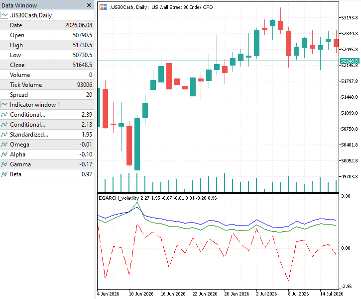
The conditional variance is plotted in blue, and the conditional volatility is depicted in green. The red-dashed plot is the standardized residuals. The indicator also exposes the volatility parameter values of the model via the last four indicator buffers.
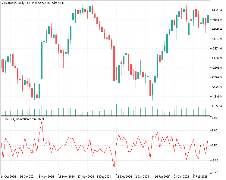
The EGARCH Innovation Z-Score measures directional market strain by normalizing raw standardized residuals relative to their theoretical conditional distribution bounds. Unlike traditional price-based oscillators, which suffer from lag and ignore changing risk regimes, the EIZ dynamically standardizes the current price shock against the symbol's current volatility floor. A reading below -2 indicates a downside innovation significantly more severe than the market anticipated, signaling a potential bottom.
// Fit EGARCH model via maximum likelihood optimization
ArchModelResult result = full_model.fit();
if(!result.conditional_volatility.Size())
  {
   Print("Model fit error ");
   return 0;
  }

// Extract full vector of standardized residuals (innovations divided by fitted volatility)
stdresid = result.std_resid();

// Slice out the dynamic evaluation window (last WindowLen entries) from standardized residuals
window = np::sliceVector(stdresid, long(stdresid.Size() - WindowLen));

// Calculate local Z-score of the most recent innovation over the sliced window (with epsilon to prevent division by zero)
EizBuffer[shift] = (window[window.Size() - 1] - window.Mean()) / (window.Std() + 1.e-8);
The indicator is shown below.
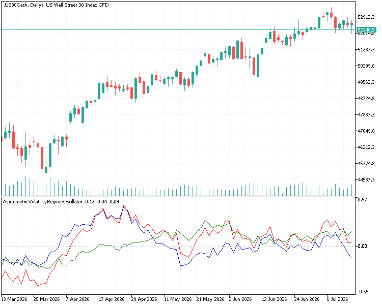
The Asymmetric Volatility Regime Oscillator (AVRO) tracks directional trend strength by monitoring the speed at which variance transitions between a calm state and a panic state. It achieves this by calculating the rolling difference between short-term and long-term averages of the EGARCH leverage component. Since gamma is typically negative for leverage-heavy assets, a consistently falling or deeply negative AVRO maps accelerating downside price velocity coupled with a structural expansion in market panic, validating short trends. Conversely, when the AVRO turns positive and begins to climb, it suggests that positive returns are suppressing market variance faster than historical norms, indicating an emerging uptrend.
// Extract full vector of standardized residuals
stdresid = result.std_resid();

// Populate fast and slow evaluation windows from the tail of standardized residuals
for(ulong i = 0; i < FastWindowLen; ++i)
   fastwindow[i] = stdresid[HistoryLen - FastWindowLen + i];
for(ulong i = 0; i < SlowWindowLen; ++i)
   slowwindow[i] = stdresid[HistoryLen - SlowWindowLen + i];

// Compute local mean values and derive the oscillator buffer (AVRO)
FastBuffer[shift] = fastwindow.Mean();
SlowBuffer[shift] = slowwindow.Mean();
AvroBuffer[shift] = FastBuffer[shift] - SlowBuffer[shift];
The red line is the short-term average of the standardized residuals, and the green line is the longer-term average standardized residuals. The blue line is the difference between the short and long-term averaged residuals. The indicator could be further improved by taking the fast and slow exponential moving averages, thereby putting more emphasis on recent volatility states.
Conclusion
This text has illuminated the nature of the constraints imposed on GARCH parameter values during the estimation process. Through a reproducible example, we demonstrated how GARCH parameters can sometimes be inhibited from taking values that accurately reflect the true nature of the data, thereby reinforcing the ingenuity of the Exponential GARCH (EGARCH) framework. With the addition of the `CEgarchProcess` class, MQL5 developers can now leverage the flexibility offered by EGARCH conditional volatility models.
The implementation of convenient utilities to quickly test for the existence of leverage effects helps practitioners avoid significant guesswork when configuring their models. Furthermore, indicators such as the EGARCH Innovation Z-Score and the Asymmetric Volatility Regime Oscillator introduce a fresh approach to market analysis. The source code for all programs referenced in this text is attached below and is also available on MQL5 Algo Forge.
| MQL5/Include/egarch/np.mqh. | Header file of various vector and matrix utility functions. |
| MQL5/Include/egarch/Arch. | Folder of header files for the conditional volatility modeling library. |
| MQL5/Files/egarch/SPY2017.csv. | This file contains S&P 500 OHLC data used in the scripts. |
| MQL5/Scripts/egarch/GARCH_ParameterPositivityLimitation.mq5. | This script generates the News Impact Curves graphic mentioned in the article. |
| MQL5/Scripts/egarch/EGARCH_Demo.mq5. | This script demonstrates fitting an EGARCH model to a dataset. |
| MQL5/Scripts/egarch/TestsForAsymmetry.mq5. | The script demonstrates the difference in asymmetric volatility inherent in forex and equity data sets. |
| MQL5/Indicators/egarch/AsymmetricVolatilityRegimeOscillator.mq5. | This is the Asymmetric Volatility Regime Oscillator source code. |
| MQL5/Indicators/egarch/EGARCH_InnovationZscore.mq5. | This is the EGARCH Innovation Z-Score source code. |
| MQL5/Indicators/egarch/EGARCH_volatility.mq5. | This is the EGARCH Volatility indicator's source code. |
The archive organizes source files into a folder structure that mirrors a local MetaTrader 5 MQL5 directory. Copy the contents of the archive's MQL5 subfolders (Include, Files, Scripts, Indicators) into their corresponding local MQL5 subfolders, preserving the `egarch` directory structure. Once copied, each file will appear within an `egarch` directory in MetaEditor.
Warning: All rights to these materials are reserved by MetaQuotes Ltd. Copying or reprinting of these materials in whole or in part is prohibited.
This article was written by a user of the site and reflects their personal views. MetaQuotes Ltd is not responsible for the accuracy of the information presented, nor for any consequences resulting from the use of the solutions, strategies or recommendations described.
 A Trailing Stop Engine in MQL5 Supporting Five Trail Methods Simultaneously
 Elite Crystal Evolution Algorithm (CEO-inspired): Practical Implementation
 Neural Networks in Trading: Adaptive Periodic Segmentation (LightGTS)
 Feature Engineering for ML (Part 12): Fractal Features in MQL5

- Free trading apps
- Over 8,000 signals for copying
- Economic news for exploring financial markets
You agree to website policy and terms of use