

协方差矩阵自适应演化策略(CMA-ES)
 170
170
 0
0

目录
概述
优化领域有很多算法,但我们正在寻找最强大的算法来解决我们交易机器人的优化问题。CMA-ES(协方差矩阵自适应演化策略)是数学严谨性与生物学直觉相结合的罕见例子之一,它创造了一种算法,该算法不仅能解决优化问题,还能学习理解问题的结构。
CMA-ES 的历史始于 20 世纪 90 年代末的德国研究实验室,当时尼古劳斯·汉森(Nikolaus Hansen)和安德烈亚斯·奥斯特迈尔(Andreas Ostermeier)提出了一个根本性问题:有没有可能设计一种优化算法,它不仅能简单地搜索解决方案,还能根据问题的具体结构进行调整?传统的进化算法在父代个体周围的球形区域内生成后代,这种方法对于简单函数效果良好,但对于复杂且条件数较差的病态问题则效果不佳。让我们一起来看一下这个有趣的算法。
算法的实现
想象一下在一个形状不规则的岛屿上寻找宝藏。通常的做法是向各个方向均匀搜索,就像岛屿是圆形的那样。CMA-ES 逐渐了解岛屿的形状,并逐渐将其搜索方向转向找到宝藏的可能性更高的方向。此外,它还能记住成功的路线,并利用这一记忆来规划未来的搜索路径。
CMA-ES 基于一个看似简单的方程: x_k ~ N(m, σ²C) 。然而,这种简洁的背后隐藏着深厚的数学结构。这里的每个符号都承载着关于搜索状态的重要信息:m 是当前对最优解位置的最佳猜测, σ 是我们愿意冒险偏离已知解的程度度量,而 C 是一个协方差矩阵,它编码了我们对函数几何特性的理解。我们唯一可以合理引入的改动是用幂律分布替换正态分布,这意味着实现将遵循一个修改后的方程:x_k ~ PowerDist(m, σ²C)。 这一修改改变了对搜索空间的探索方式(更大的‘跳跃’),但保留了算法的基本自适应性质。
协方差矩阵 C 是该算法的真正核心。它起初是一个不起眼的单位矩阵,代表一种球形分布。但每一次迭代都会有所演变,在快速改进的方向上不断延伸,而在进展缓慢的地方则有所收缩。逐渐地,球体变成一个椭圆,然后变成一个细长的椭球体,理想情况下,其方向与待优化函数的轮廓相一致。
CMA-ES 的主要创新之处在于演化路径的概念。这是算法的一种遗传记忆,它不仅记得成功点在哪里,还记得算法是如何找到这些点的。进化路径累积了关于连续成功步骤的信息,形成了一个指向最有前景搜索区域的方向向量。第二条进化路径执行着更为精细的功能:它控制着步长。如果算法的连续步骤之间存在相关性,即每个后续步骤都延续了前一个步骤的方向,那么步长就会增加 — 算法“感觉”它正在朝着正确的方向前进。如果步骤是随机的且不相关,则步长减小 — 或许算法已经接近最优解,需要更仔细地进行搜索。
在 CMA-ES 中,进化的生物学隐喻背后隐藏着一条严谨的数学原理 — 最大似然估计。该算法会不断地问自己:哪些分布参数使得观察到的成功点最有可能出现?这将进化优化从一种启发式方法转变为一种基于统计的方法。
C 协方差矩阵的每次更新都包含两个部分:基于进化路径的秩一更新和使用来自整个选定种群的信息的秩 μ更新。秩一更新提供了稳定性和捕捉长期趋势的能力,而秩μ更新则允许快速适应当前一代的新信息。
在 CMA-ES 的背景下,使用了一个修改后的 Heaviside 函数,该函数在该算法的停滞检测机制中起着重要作用。该函数将进化路径的长度与预期长度进行比较;如果路径过短,则表明存在“随机摇摆”的情况。 停用条件(hsig = 0):算法随机“游荡”,步长相互抵消,则步长可能过大。在停滞期,秩一更新的影响会减弱,我们会更多地依赖来自整体群体的信息。 激活条件(hsig = 1): 算法朝着某个方向发展,连续的步骤相互关联,那么步长就足以适应当前情况。
CMA-ES 最深刻的特性之一是它对搜索空间变换的不变性。该算法同样有效地求解函数 f(x) 和函数 f(Ax + b),其中 A 是任意非奇异矩阵,b 是任意移位向量。这意味着 CMA-ES 与坐标系的选择无关。这种不变性并非偶然;它是使用最大似然原则和调整协方差矩阵的直接结果。该算法能自动为问题检测出一个自然坐标系,其中坐标轴与函数变化的主要方向一致。
理论上的优雅必须兼顾实际可用性。CMA-ES 需要 O(n²) 内存来存储协方差矩阵,需要 O(n³) 计算来进行特征值分解,这使得该算法适用于维度高达数百个变量的问题。对于大维度情况,已经开发出了专门的改进方法:sep-CMA-ES 仅限于对角协方差矩阵,VkD-CMA 使用可变维度,而 LM-CMA 则应用了有限记忆原理。这些方法的实现目前不在本文讨论范围内,但后续文章中可能会再次探讨。
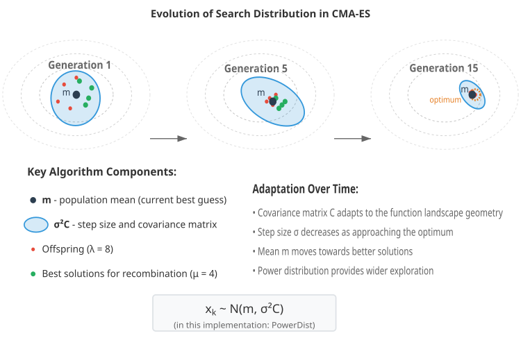
图1.CMA-ES 算法示意图
该图展示了算法经过几代演变的过程 — 三个算法状态的快照(第 1 代、第 5 代和第 15 代),展示了种群如何逐渐收敛到最优解。
协方差矩阵的调整 — 蓝色椭圆显示了当代数变化时分布形状的变化: 1-圆形(单位矩阵),5-拉长和旋转,15-根据局部几何形状进行精细调整。
算法组成: 红点代表整个种群(λ 个后代),绿点代表最佳解(μ 个父代),黑点 m 代表种群均值,虚线圆圈代表目标函数的等值线。
关键公式如下,并附有关于幂律修正的说明。该图清晰地展示了算法如何根据待优化函数的形态调整其搜索策略,逐步缩小搜索空间并逼近最优解。
让我们来编写伪代码。
初始化
- 设置算法参数:
- 种群规模(lambda)= 50
- 父母数量 (mu) = 25
- 秩-1 更新的学习率(c1)= 0.01
- 秩-μ 更新的学习率(cμ)= 0.8
- 步长阻尼 = 0.6
- 初始步长(sigma)= 0.3
- 计算重组权重:
- 对于每个 μ 个父代,计算其权重为 log(μ + 0.5) - log(i + 1)
- 将权重归一化,使其总和等于 1。
- 计算有效选择质量 μ_eff(由重组权重决定的等效规模)
- 初始化策略参数:
- 计算进化路径(cs,cc)的学习率
- 计算标准正态向量(chiN)的期望范数
- 确定特征值分解的区间
- 初始化数据结构:
- C 协方差矩阵 = 单位矩阵
- 特征向量矩阵 B = 单位矩阵
- 特征值向量 D = 单位向量
- pc 和 ps 演化路径 = 零向量
- 总体均值 m = 搜索空间中的随机点
- 创建初始种群:
- 在搜索空间中生成 lambda 随机点
演化的基本循环
重复此过程直至达到停止条件:
第 1 步:产生后代
- 对于每个 lambda 后代:
- 从标准正态分布生成随机向量 z
- 应用变换:y = B × D × z
- 创建后代:x_k = m + σ × y
- 对 x_k 应用搜索空间约束
第 2 步:评估和更新
- 评估所有后代的适应度
- 对种群进行排序:
- 按适应度降序排列后代
- 如有必要,更新已找到的最佳解决方案。
- 更新种群均值:
- 存储先前的平均值 m_old
- 计算新的均值,即 μ 个最佳后代的加权和:m_new = Σ(w_i × x_i),其中 i 从 1 到 μ
- 更新进化路径:
- 计算均值偏移:y_w = (m_new - m_old) / σ
- 利用特征值分解计算 C^(-1/2) × y_w
- 更新演化路径,步长为:ps = (1 - cs) × ps + √(cs × (2 - cs) × μ_eff) × C^(-1/2) × y_w
- 检查停滞条件(Heaviside函数)
- 更新协方差矩阵的演化路径:pc = (1 - cc) × pc + stagnation_indicator × √(cc × (2 - cc) × μ_eff) × y_w
- 更新协方差矩阵:
- 根据向量 pc 的外积准备秩-1 更新
- 根据最佳子代偏差的加权和,准备秩-μ 更新
- 更新 C:C = (1 - c1 - cμ) × C + c1 × (pc × pc^T) + cμ × Σ(w_i × y_i × y_i^T)
- 确保矩阵对称性
- 更新步长:
- 基于 ps 路径长度计算自适应系数
- 更新 σ:σ = σ × exp((cs/damps) × (||ps||/chiN - 1))
- 为了保证数值稳定性,应将 σ 限制在合理的范围内。
- 特征值分解(如有必要):
- 如果自上次分解以来已经经过了足够多的迭代:
- 对 C = B × D² × B^T 进行雅可比分解
- 按降序排列特征值和特征向量
- 确保矩阵的正定性
- 如果自上次分解以来已经经过了足够多的迭代:
- 检查并修正协方差矩阵:
- 定期检查 C 正定性
- 如有必要,在对角线上增加一个较小的数值。
- 确保矩阵对称性
现在,让我们编写从 C_AO 类派生的 C_AO_CMAES,它将实现 CMA-ES 优化算法。
公有成员与方法:
- SetParams() - 从以下位置设置 CMA-ES 参数值 参数数组。
- Init() - 初始化算法。接受每个变量的最小值、最大值和步长,以及轮数。
- Moving() -实现算法的主循环,负责生成新的解决方案。
- Revision() - 评估新解决方案并更新算法状态。
私有字段:
- CMA-ES 参数 - 变量 包含 CMA-ES 算法的具体参数:父代数量 (mu)、步长 (sigma)、学习率 (learningRateC1, learningRateCMu)、阻尼因子(stepSizeDamping)以及其他算法运行所必需的参数。
- CMA-ES数据结构- 数组用于存储重组权重、covMatrix 协方差矩阵、B 特征向量、D 特征值、进化路径(pc,ps)以及其他辅助数据。mu_eff、counteval、eigeneval、chiN、eigenInterval 值用于控制和管理算法进度。
- 用于性能优化的变量旨在加快算法运行过程中的计算速度,如学习率和阻尼。
- 辅助数组 在执行各种操作时,用作向量和矩阵的临时存储。
- 辅助方法执行 CMA-ES 算法的各个步骤,例如初始化分布、更新分布、计算特征分解、对种群进行排序、计算权重、更新均值、检查正定性以及确保正定性。
总的来说, C_AO_CMAES 该类封装了 CMA-ES 算法的逻辑,提供了初始化、参数调整和执行优化的接口。它包含了实现算法所需的参数、数据数组和方法。公有与私有成员的划分有助于控制对类内部组件的访问。
//————————————————————————————————————————————————————————————————————
class C_AO_CMAES : public C_AO
{
  public: //----------------------------------------------------------
  ~C_AO_CMAES () { }
  C_AO_CMAES ()
  {
    ao_name = "CMAES";
    ao_desc = "Covariance Matrix Adaptation Evolution Strategy";
    ao_link = "https://www.mql5.com/en/articles/18227";

    // Default parameters
    popSize         = 50;          // Default population size (lambda)
    mu              = 25;          // Number of parents (half of the population)
    learningRateC1  = 0.01;        // Learning rate for rank-1 update
    learningRateCMu = 0.8;         // Learning rate for rank-μ update
    stepSizeDamping = 0.6;         // Damping for step size

    // Create and initialize the parameters array
    ArrayResize (params, 5);
    params [0].name = "popSize";         params [0].val = popSize;
    params [1].name = "mu";              params [1].val = mu;
    params [2].name = "learningRateC1";  params [2].val = learningRateC1;
    params [3].name = "learningRateCMu"; params [3].val = learningRateCMu;
    params [4].name = "stepSizeDamping"; params [4].val = stepSizeDamping;
  }

  void SetParams ()
  {
    popSize         = (int)params [0].val;
    mu              = (int)params [1].val;
    learningRateC1  = params      [2].val;
    learningRateCMu = params      [3].val;
    stepSizeDamping = params      [4].val;
  }

  bool Init (const double &rangeMinP  [],  // minimum values
             const double &rangeMaxP  [],  // maximum values
             const double &rangeStepP [],  // step size
             const int     epochsP = 0);

  void Moving   ();
  void Revision ();

  //------------------------------------------------------------------
  private: //---------------------------------------------------------
  // CMA-ES specific parameters
  int mu;                  // Number of parents (selected points)
  double sigma;            // Step size
  double learningRateC1;   // Learning rate for rank-1 update
  double learningRateCMu;  // Learning rate for rank-μ update
  double stepSizeDamping;  // Damping factor for step size update

  // CMA-ES specific data structures
  double weights   [];      // Recombination weights
  double covMatrix [];      // Covariance matrix (stored as a one-dimensional array)
  double B  [];             // C eigenvectors
  double D  [];             // C eigenvalues (square roots)
  double pc [];             // Evolution path for C
  double ps [];             // Evolution path for step-size control
  double mu_eff;            // Effective selection mass
  int    counteval;         // Counter of function evaluations since the last decomposition
  int    eigeneval;         // Generation counter when decomposition was performed
  double chiN;              // Expected norm N(0,I)
  int    eigenInterval;     // Interval for eigenvalue decomposition

  // Variables for performance optimization
  double cs;                // Learning rate for the sigma path
  double cc;                // Learning rate for rank-1 path
  double damps;             // Damping for sigma
  double hsig_threshold;    // Threshold for the Heaviside function

  // Auxiliary arrays
  double y_vec     [];         // Mutation vector
  double arindex   [];         // Array of indices for sorting
  double arfitness [];         // Fitness array for sorting
  double temp_vec  [];         // Temporary vector for matrix operations
  double invsqrtC_times_yw []; // Temporary storage for C^(-1/2) * y_w

  // Caching variables for Box-Muller
  double cached_normal;
  bool   has_cached;

  // Auxiliary methods
  void   InitDistribution          ();
  void   UpdateDistribution        ();
  void   ComputeEigendecomposition ();
  double GetChiN                   ();
  void   SortPopulation            ();
  void   ComputeWeights            ();
  void   UpdateMean                ();
  bool   CheckPositiveDefinite     ();
  void   EnforcePositiveDefinite   ();
};
//————————————————————————————————————————————————————————————————————
C_AO_CMAES 类的 Init 方法初始化 CMA-ES 算法。它以最小和最大参数值、步长和迭代次数作为输入。首先,调用 StandardInit 方法执行标准初始化。has_cached 标志初始化为 “false”,表示 Box-Muller 随机数生成没有缓存值。接下来,将 sigma 步长初始化为初始值 0.3(搜索范围的 30%)。调用 ComputeWeights 方法来计算重组权重,调用 GetChiN 方法来计算期望范数 N(0, I)。
cs、cc、damps 和 hsig_threshold 参数是根据 mu_eff(有效质量)和坐标数(coords)计算的。这些参数用于在运行过程中调整 CMA-ES 策略。计算并设置 eigenInterval,以确定执行特征值分解的频率。此参数用于优化性能。
内存被分配给 CMA-ES 特有的数组,例如 covMatrix 协方差矩阵、B 特征向量、D 特征值、pc 和 ps 演化路径、y_vec、arindex、arfitness、temp_vec 和 invsqrtC_times_yw 时间向量。仅当需要更改问题维度时,才会重新创建数组。
pc 和 ps 演化路径数组初始化为零,covMatrix 协方差矩阵和 B 特征向量矩阵初始化为单位矩阵,D 特征值数组初始化为 1。调用 InitDistribution 方法来初始化初始分布。然后重置 counteval 和 eigeneval 函数的评估计数器。“revision” 标志设置为 “true” 表示应重新计算适应度值。“true” 表示初始化成功。
总之,Init 方法执行 CMA-ES 算法工作所需的所有初始化操作,包括设置参数、为数组分配内存和初始化初始值。
//————————————————————————————————————————————————————————————————————
bool C_AO_CMAES::Init (const double &rangeMinP [],  // minimum values
                       const double &rangeMaxP [],  // maximum values
                       const double &rangeStepP [], // step size
                       const int     epochsP = 0)   // number of epochs
{
  if (!StandardInit (rangeMinP, rangeMaxP, rangeStepP)) return false;

  //------------------------------------------------------------------
  // Initialize Box-Muller caching
  has_cached = false;

  // Initialize CMA-ES specific variables
  sigma          = 0.3;  // Initial step size (30% of search range)

  // Calculate the effective mass of the variance selection
  ComputeWeights ();

  // Expected norm N(0,I)
  chiN = GetChiN ();

  // Calculate and save strategy parameters
  cs = (mu_eff + 2.0) / (coords + mu_eff + 5.0);
  cc = (4.0 + mu_eff / coords) / (coords + 4.0 + 2.0 * mu_eff / coords);
  damps = 1.0 + 2.0 * MathMax (0.0, MathSqrt ((mu_eff - 1.0) / (coords + 1.0)) - 1.0) + cs;
  hsig_threshold = 1.4 + 2.0 / (coords + 1.0);

  // Set the eigenvalue decomposition interval - tuning for performance
  eigenInterval = (int)(coords / (10.0 * MathSqrt (learningRateC1 + learningRateCMu)));
  eigenInterval = MathMax (1, eigenInterval);

  // Allocate arrays only once
  ArrayResize (covMatrix, coords * coords);
  ArrayResize (B, coords * coords);
  ArrayResize (D, coords);
  ArrayResize (pc, coords);
  ArrayResize (ps, coords);
  ArrayResize (y_vec, coords);
  ArrayResize (arindex, popSize);
  ArrayResize (arfitness, popSize);
  ArrayResize (temp_vec, coords);
  ArrayResize (invsqrtC_times_yw, coords);

  // Initialize evolution paths with zeros
  ArrayInitialize (pc, 0);
  ArrayInitialize (ps, 0);

  // Fast initialization of the identity covariance matrix and decomposition
  ArrayInitialize (covMatrix, 0.0);
  ArrayInitialize (B, 0.0);

  for (int i = 0; i < coords; i++)
  {
    covMatrix [i * coords + i] = 1.0;
    B [i * coords + i] = 1.0;
    D [i] = 1.0;
  }

  // Initialize initial distribution
  InitDistribution ();

  // Reset calculation counters
  counteval = 0;
  eigeneval = 0;

  // Forced fitness recalculation
  revision = true;

  return true;
}
//————————————————————————————————————————————————————————————————————
C_AO_CMAES 类中的 Moving 方法负责在种群中生成新的后代(解)。 变换 y = B * D * z:在遍历种群的循环中,有一个嵌套循环,该循环遍历每个个体的所有坐标。计算每个坐标 i 处的 y_vec [i] 值。这是通过矩阵乘法实现的。实际上,它是将 z 个随机数的向量乘以矩阵 “B * D”,其中 B 是协方差矩阵的特征向量,D 是协方差矩阵的特征值,z 是使用 u.PowerDistribution 函数生成的随机数。
后代生成:计算每个 k 个后代的每个 i 坐标的 (a [k].c [i]) 值。这是通过将缩放向量 y_vec[i] 添加到当前均值 cB[i](当前分布的中心)来实现的。缩放是通过将 y_vec[i] 乘以 'sigma' 步长来实现的。因此,a[k].c[i] = cB[i] + sigma * y_vec[i]。
u.SeInDiSp 函数确保子代的坐标值保持在 rangeMin[i]、rangeMax[i] 和 rangeStep[i] 定义的有效范围内。它可以对值进行裁剪,使其在边界处反弹,并将其量化到最接近的有效步长值。生成所有后代后,“revision” 标志设置为 “true”,并且应该重新计算生成的后代的适应度值。
因此,该方法 根据当前分布生成新的解集( cB 平均值和协方差矩阵,表示为B 和 D) 和 sigma 步长。它使用随机数在当前均值附近产生微小变化,以探索搜索空间。这 SeInDiSp 函数确保新解保持在允许的范围内,以及 “revision” 标志。 以便随后重新评估这些新解的适应度。
//————————————————————————————————————————————————————————————————————
void C_AO_CMAES::Moving ()
{
  // Generate new lambda descendants
  for (int k = 0; k < popSize; k++)
  {

    // Apply the transformation y = B*D*z
    for (int i = 0; i < coords; i++)
    {
      y_vec [i] = 0.0;
      for (int j = 0; j < coords; j++)
      {
        y_vec [i] += B [i * coords + j] * D [j] * u.PowerDistribution (0.0, -8, 8, 20);
      }

      // Generate a descendant: x_k = m + σ * y
      a [k].c [i] = cB [i] + sigma * y_vec [i];
      a [k].c [i] = u.SeInDiSp (a [k].c [i], rangeMin [i], rangeMax [i], rangeStep [i]);
    }
  }

  // Fitness recalculation mark
  revision = true;
}
//————————————————————————————————————————————————————————————————————
C_AO_CMAES 类的 Revision 方法负责在评估新种群的适应度函数后更新算法参数。首先,该方法检查 “revision” 标志的值。然后,调用 SortPopulation() 方法,对当前种群进行排序,使最好的个体位于顶部。UpdateDistribution() 方法根据种群中最佳个体的信息来更新 CMA-ES 分布的参数(策略向量的 cB 均值、协方差矩阵、sigma 步长、进化路径)。分布更新是 CMA-ES 的一个关键步骤,因为它允许算法根据获得的结果调整其搜索策略。
因此,Revision 方法代表了 CMA-ES 的主要适应周期。它对种群进行排序,根据最优个体更新分布参数,并增加计算计数器的数值。
//————————————————————————————————————————————————————————————————————
void C_AO_CMAES::Revision ()
{
  if (!revision) return;

  revision = false;

  // Sort the population by fitness
  SortPopulation ();

  // Update distribution parameters based on selected individuals
  UpdateDistribution ();

  // Update the calculation counter
  counteval++;
}
//————————————————————————————————————————————————————————————————————
C_AO_CMAES 类的 InitDistribution 方法旨在初始化解决方案搜索的初始分布。该方法为搜索空间中的每个坐标确定一个初始均值(cB)。对于每个坐标 i,使用 u.RNDfromCI() 在 rangeMin[i] 和 rangeMax[i] 之间随机设置 cB[i] 的值。外层循环遍历整个种群(popSize 个个体)。在这个循环内部,有一个内循环,用于遍历每个个体的所有坐标。为每个后代生成坐标。首先,它们从给定的范围 RNDfromCI 中随机选择,然后使用 SeInDiSp 四舍五入到采样步长。
u.RNDfromCI 函数生成给定区间内均匀分布的随机数。u.SeInDiSp 函数确保每个个体的生成坐标都位于由定义的可接受范围内。 rangeMin[i]、rangeMax[i] 和 rangeStep [i].
该方法使用在搜索空间中均匀分布的随机解来初始化初始种群。分布中心(cB)也是随机选择的。这为 CMA-ES 的后续迭代提供了一个起点,算法将调整搜索策略以找到最优解。
//+------------------------------------------------------------------+
//| Initialize search distribution                                   |
//+------------------------------------------------------------------+
void C_AO_CMAES::InitDistribution ()
{
  // Set the initial mean to the center of the search space
  for (int i = 0; i < coords; i++)
  {
    cB [i] = u.RNDfromCI (rangeMin [i], rangeMax [i]);
  }

  for (int k = 0; k < popSize; k++)
  {
    for (int i = 0; i < coords; i++)
    {
      // Generate a uniformly distributed point
      a [k].c [i] = u.RNDfromCI (rangeMin [i], rangeMax [i]);
      a [k].c [i] = u.SeInDiSp (a [k].c [i], rangeMin [i], rangeMax [i], rangeStep [i]);
    }
  }
}
//————————————————————————————————————————————————————————————————————
GetChiN 方法计算从 N (0,I) 中抽取的随机向量的期望范数,给定坐标数 ( coords )。 。结果根据搜索空间的维度进行近似计算。
//+------------------------------------------------------------------+
//| Calculate the expected norm N(0,I)                               |
//+------------------------------------------------------------------+
double C_AO_CMAES::GetChiN ()
{
  double n = (double)coords;
  return MathSqrt (n) * (1.0 - 1.0 / (4.0 * n) + 1.0 / (21.0 * n * n));
}
//————————————————————————————————————————————————————————————————————
SortPopulation 旨在根据目标函数值(适应度)对一组解决方案进行排序,以确定最佳解决方案。首先,该方法将种群中每个个体的适应度值复制到 arfitness 辅助数组中。同时创建了 arindex 数组,该数组最初包含个体的索引。这是必要的,以便在按适应度排序后,能够恢复排序后的适应度与种群中原始个体之间的对应关系。
采用插入排序算法。它遍历 arfitness 数组,对于每个元素,将其插入到数组已排序部分的正确位置,并将较大的元素向右移动。值得注意的是,排序是按降序进行的(在 “while” 循环中 arfitness [j] < tempFitness),目标是最大化目标函数(fitness)。与 arfitness 一起,arindex 也同步排序,以跟踪个体原始索引的位置。
排序后,该方法检查最佳个体的适应度是否优于当前最佳解,如果是,则更新 fB,并将最佳解替换为种群中最佳个体的坐标。因此,该方法不仅根据适应度对种群进行排序,还能记录当前找到的最佳解。
//+------------------------------------------------------------------+
//| Sort the population by fitness                                   |
//+------------------------------------------------------------------+
void C_AO_CMAES::SortPopulation ()
{
  // Copy fitness values and indices
  for (int i = 0; i < popSize; i++)
  {
    arindex [i] = i;
    arfitness [i] = a [i].f;
  }

  for (int i = 1; i < popSize; i++)
  {
    double tempFitness = arfitness [i];
    double tempIndex = arindex [i];
    int j = i - 1;

    // Sort in descending order (for maximization)
    while (j >= 0 && arfitness [j] < tempFitness)
    {
      arfitness [j + 1] = arfitness [j];
      arindex [j + 1] = arindex [j];
      j--;
    }

    arfitness [j + 1] = tempFitness;
    arindex [j + 1] = tempIndex;
  }

  // Update the best solution if necessary
  if (arfitness [0] > fB)
  {
    fB = arfitness [0];
    int bestIdx = (int)arindex [0];
    ArrayCopy (cB, a [bestIdx].c, 0, 0, coords);
  }
}
//————————————————————————————————————————————————————————————————————
UpdateMean 方法通过加权重组最优个体来更新群体均值(cB)。对于每个坐标,计算一个新的平均值,该平均值是来自最优个体的加权坐标值之和,其中权重在 weights 数组中指定。
//+------------------------------------------------------------------+
//| Update the mean using weighted recombination                     |
//+------------------------------------------------------------------+
void C_AO_CMAES::UpdateMean ()
{
  // Weighted recombination: m^(g+1) = Σ w_i * x_{i:λ}^(g+1)
  for (int j = 0; j < coords; j++)
  {
    double meanSum = 0.0;
    for (int i = 0; i < mu; i++)
    {
      int idx = (int)arindex [i];
      meanSum += weights [i] * a [idx].c [j];
    }
    cB [j] = meanSum;
  }
}
//————————————————————————————————————————————————————————————————————
ComputeWeights 方法用于计算加权重组的权重,按大小 mu 分配权重数组,并计算 log(mu+0.5) 以用于权重公式。对于从 0 到 mu-1 的每个 i,它将 log(mu + 0.5) 与 log(i+1) 之间的差值赋给一个权重,将这些权重相加,该方法将所有权重除以该和,使和等于 1,然后计算权重的平方和,计算 mu_eff — 使用权重的效率,这对于调整算法的速度和方差非常重要。
该方法考虑了最佳解的贡献,为重组提供了最优权重。
//+------------------------------------------------------------------+
//| Calculate weighted recombination weights                         |
//+------------------------------------------------------------------+
void C_AO_CMAES::ComputeWeights ()
{
  // Allocate the array of weights
  ArrayResize (weights, mu);

  // Pre-calculate log(mu + 0.5)
  double log_mu_plus_half = MathLog (mu + 0.5);

  // Calculate positive weights
  double sum = 0.0;
  for (int i = 0; i < mu; i++)
  {
    weights [i] = log_mu_plus_half - MathLog (i + 1);
    sum += weights [i];
  }

  // Normalize weights
  double sum_weights = 0.0;
  double sum_squares = 0.0;
  for (int i = 0; i < mu; i++)
  {
    weights [i] /= sum;
    sum_weights += weights [i];
    sum_squares += weights [i] * weights [i];
  }

  // Calculate the effective mass of the variance selection
  mu_eff = sum_weights * sum_weights / sum_squares;
}
//————————————————————————————————————————————————————————————————————
UpdateDistribution 方法更新分布参数,即 CMA-ES 算法中的协方差矩阵(covMatrix)和步长(sigma)。如果经过足够多的世代(counteval - eigeneval > eigenInterval),则计算特征值分解,并将当前均值(cB)存储在 oldMean 临时数组中。该方法调用 UpdateMean 来计算新的均值,计算新均值与旧均值之差除以 sigma,并将 y_w 乘以 C^(-1/2),使用 B 和 D 分解将其分解为几个步骤,并将结果存储在 invsqrtC_times_yw 中。
然后,该方法使用 invsqrtC_times_yw 更新 ps 步长的演化路径,根据 ps 范数和预期长度确定进展是否被认为是“停滞的”,然后使用 y_w 和 hsig 进展指标更新 pc 协方差矩阵的演化路径。该方法首先计算 c1a 秩一更新矩阵,然后基于个体与旧均值之差除以 sigma,使用 “weights” 计算 cmu 秩μ更新矩阵,使用秩一和秩 μ更新来更新 covMatrix 协方差矩阵,并在进展停滞时调整 c1。定期调用 EnforcePositiveDefinite 函数,以确保协方差矩阵为正定矩阵。sigma 步长根据 ps 范数进行更新,并且为了数值稳定性,其值被限制在 min_sigma 和 max_sigma 之间。
一般来说, UpdateDistribution 根据搜索历史(进化路径)和种群数据调整分布参数(协方差矩阵和步长),以适应目标函数的地形。
//+------------------------------------------------------------------+
//| Update distribution parameters                                   |
//+------------------------------------------------------------------+
void C_AO_CMAES::UpdateDistribution ()
{
  // Check the necessity of eigenvalue decomposition
  if (counteval - eigeneval > eigenInterval)
  {
    ComputeEigendecomposition ();
    eigeneval = counteval;
  }

  // Preserve the old average
  double oldMean [];
  ArrayResize (oldMean, coords);
  ArrayCopy (oldMean, cB, 0, 0, coords);

  // Update average
  UpdateMean ();

  // Calculate the mean shift
  double y_w [];
  ArrayResize (y_w, coords);
  for (int j = 0; j < coords; j++)
  {
    y_w [j] = (cB [j] - oldMean [j]) / sigma;
  }

  // Calculate C^(-1/2) * y_w
  // Step 1: B^T * y_w
  ArrayInitialize (temp_vec, 0.0);
  for (int i = 0; i < coords; i++)
  {
    for (int j = 0; j < coords; j++)
    {
      temp_vec [i] += B [j * coords + i] * y_w [j];
    }
  }

  // Step 2: D^(-1) * (B^T * y_w)
  for (int i = 0; i < coords; i++)
  {
    temp_vec [i] /= D [i];
  }

  // Step 3: B * D^(-1) * B^T * y_w
  ArrayInitialize (invsqrtC_times_yw, 0.0);
  for (int i = 0; i < coords; i++)
  {
    for (int j = 0; j < coords; j++)
    {
      invsqrtC_times_yw [i] += B [i * coords + j] * temp_vec [j];
    }
  }

  // Update the evolution path for sigma
  double norm_ps_squared = 0.0;
  for (int i = 0; i < coords; i++)
  {
    ps [i] = (1.0 - cs) * ps [i] + MathSqrt (cs * (2.0 - cs) * mu_eff) * invsqrtC_times_yw [i];
    norm_ps_squared += ps [i] * ps [i];
  }

  // Heaviside function
  double norm_ps = MathSqrt (norm_ps_squared);
  double expected_length = MathSqrt (1.0 - MathPow (1.0 - cs, 2.0 * counteval)) * chiN;
  bool hsig = norm_ps / expected_length < hsig_threshold;

  // Update the evolution path for C
  double delta_hsig = hsig ? 1.0 : 0.0;
  for (int i = 0; i < coords; i++)
  {
    pc [i] = (1.0 - cc) * pc [i] + delta_hsig * MathSqrt (cc * (2.0 - cc) * mu_eff) * y_w [i];
  }

  // Prepare rank-1 update
  double c1a [];
  ArrayResize (c1a, coords * coords);
  for (int i = 0; i < coords; i++)
  {
    for (int j = 0; j <= i; j++)
    {
      c1a [i * coords + j] = c1a [j * coords + i] = pc [i] * pc [j];
    }
  }

  // Prepare rank-μ update
  double cmu [];
  ArrayResize (cmu, coords * coords);
  ArrayInitialize (cmu, 0.0);

  for (int k = 0; k < mu; k++)
  {
    int idx = (int)arindex [k];

    // Calculate y_i = (x_i - m_old) / sigma
    for (int i = 0; i < coords; i++)
    {
      temp_vec [i] = (a [idx].c [i] - oldMean [i]) / sigma;
    }

    // Add the weighted outer product
    for (int i = 0; i < coords; i++)
    {
      for (int j = 0; j <= i; j++)
      {
        double update = weights [k] * temp_vec [i] * temp_vec [j];
        cmu [i * coords + j] += update;
        if (i != j) cmu [j * coords + i] += update;
      }
    }
  }

  // Update C the covariance matrix
  double c1 = learningRateC1;
  double cmu_rate = learningRateCMu;

  // Adjust c1 if hsig is 'false' (progress stalled)
  if (!hsig)
  {
    c1 *= (1.0 - (1.0 - delta_hsig) * cc * (2.0 - cc));
  }

  double one_minus_c1_cmu = 1.0 - c1 - cmu_rate;

  // Update C with rank-1 and rank-μ updates
  for (int i = 0; i < coords; i++)
  {
    for (int j = 0; j <= i; j++)
    {
      covMatrix [i * coords + j] = one_minus_c1_cmu * covMatrix [i * coords + j] +
                                   c1 * c1a [i * coords + j] +
                                   cmu_rate * cmu [i * coords + j];

      // Maintain symmetry
      if (i != j)
      {
        covMatrix [j * coords + i] = covMatrix [i * coords + j];
      }
    }
  }

  // Ensure positive definiteness
  if (counteval % (10 * eigenInterval) == 0)
  {
    EnforcePositiveDefinite ();
  }

  //  Update the sigma step size
  double exponent = (cs / damps) * (norm_ps / chiN - 1.0);
  sigma *= MathExp (exponent);

  // Limit sigma for numerical stability
  double min_sigma = 1e-16;
  double max_eigenvalue = D [0]; // D sorted in descending order
  double max_sigma = 1e4 * MathMax (1.0, MathSqrt (max_eigenvalue));

  if (sigma < min_sigma) sigma = min_sigma;
  else
    if (sigma > max_sigma) sigma = max_sigma;
}
//————————————————————————————————————————————————————————————————————
ComputeEigendecomposition 执行分解 使用改进的雅可比方法将 covMatrix 对称协方差分解为特征值和特征向量,该方法创建 covMatrix 的副本,因此不会修改原始数据。最初,B 被设置为单位矩阵,代表初始基。它会执行最大迭代次数,或者直到非对角线上的非零元素小于 “tolerance” 为止。
求最大非对角线元素:找出对角线以外绝对值最大的元素,选择该元素进行旋转。接下来,如果最大值小于 “tolerance”,则中断循环。该方法计算 phi 以执行雅可比旋转,通过应用旋转来修改 C_copy 的元素,并根据旋转更新 B 矩阵的列(特征向量)。迭代结束后,该方法求出对角元素的平方根(确保最小正性为 1e-14),并将特征值和相应的特征向量按降序排列,以供后续使用。因此,该方法能够准确计算协方差矩阵的特征值和特征向量。
//+------------------------------------------------------------------+
//| Calculate the eigenvalue decomposition using the Jacobi method   |
//+------------------------------------------------------------------+
void C_AO_CMAES::ComputeEigendecomposition ()
{
  // Create a copy of the covariance matrix for decomposition
  double C_copy [];
  ArrayResize (C_copy, coords * coords);
  ArrayCopy (C_copy, covMatrix);

  // Initialize B as the identity matrix
  for (int i = 0; i < coords; i++)
  {
    for (int j = 0; j < coords; j++)
    {
      B [i * coords + j] = (i == j) ? 1.0 : 0.0;
    }
  }

  // Improved Jacobi eigenvalue decomposition
  int max_iterations = 10; //50 * coords;
  double tolerance   = 0.01; //1e-14 * coords * coords;

  for (int iter = 0; iter < max_iterations; iter++)
  {
    // Find the largest off-diagonal element
    double max_val = 0.0;
    int p = 0, q = 1;

    for (int i = 0; i < coords - 1; i++)
    {
      for (int j = i + 1; j < coords; j++)
      {
        double val = MathAbs (C_copy [i * coords + j]);
        if (val > max_val)
        {
          max_val = val;
          p = i;
          q = j;
        }
      }
    }

    // Check convergence
    if (max_val < tolerance) break;

    // Calculate the rotation angle
    double app = C_copy [p * coords + p];
    double aqq = C_copy [q * coords + q];
    double apq = C_copy [p * coords + q];

    double phi = 0.5 * MathArctan (2.0 * apq / (aqq - app + 1e-14));
    double c = MathCos (phi);
    double s = MathSin (phi);

    // Update the matrix elements
    double app_new = c * c * app - 2 * c * s * apq + s * s * aqq;
    double aqq_new = s * s * app + 2 * c * s * apq + c * c * aqq;

    C_copy [p * coords + p] = app_new;
    C_copy [q * coords + q] = aqq_new;
    C_copy [p * coords + q] = C_copy [q * coords + p] = 0.0;

    // Update other elements in p and q rows/columns
    for (int i = 0; i < coords; i++)
    {
      if (i != p && i != q)
      {
        double aip = C_copy [i * coords + p];
        double aiq = C_copy [i * coords + q];
        C_copy [i * coords + p] = C_copy [p * coords + i] = c * aip - s * aiq;
        C_copy [i * coords + q] = C_copy [q * coords + i] = s * aip + c * aiq;
      }
    }

    // Update eigenvectors
    for (int i = 0; i < coords; i++)
    {
      double bip = B [i * coords + p];
      double biq = B [i * coords + q];
      B [i * coords + p] = c * bip - s * biq;
      B [i * coords + q] = s * bip + c * biq;
    }
  }

  // Extract eigenvalues and ensure positivity
  double min_eigenvalue = 1e-14;
  for (int i = 0; i < coords; i++)
  {
    D [i] = MathSqrt (MathMax (min_eigenvalue, C_copy [i * coords + i]));
  }

  // Sort eigenvalues and vectors in descending order
  for (int i = 0; i < coords - 1; i++)
  {
    int max_idx = i;
    for (int j = i + 1; j < coords; j++)
    {
      if (D [j] > D [max_idx]) max_idx = j;
    }

    if (max_idx != i)
    {
      // Exchange eigenvalues
      double temp = D [i];
      D [i] = D [max_idx];
      D [max_idx] = temp;

      // Exchange eigenvectors
      for (int k = 0; k < coords; k++)
      {
        temp = B [k * coords + i];
        B [k * coords + i] = B [k * coords + max_idx];
        B [k * coords + max_idx] = temp;
      }
    }
  }
}
//————————————————————————————————————————————————————————————————————
CheckPositiveDefinite 方法检查协方差矩阵是否为正定矩阵。它快速检查对角线元素的正性,并比较最小特征值(来自 D 数组按降序排列)包含一个较小的正数 1e-14 。如果两个检查都通过,则该方法返回 'true'。
//+------------------------------------------------------------------+
//| Check the positive definiteness of the covariance matrix         |
//+------------------------------------------------------------------+
bool C_AO_CMAES::CheckPositiveDefinite ()
{
  // Quick check: all diagonal elements should be positive
  for (int i = 0; i < coords; i++)
  {
    if (covMatrix [i * coords + i] <= 0) return false;
  }

  // Check if the minimum eigenvalue is positive
  double min_eigenvalue = D [coords - 1]; // D is sorted in descending order
  return min_eigenvalue > 1e-14;
}
//————————————————————————————————————————————————————————————————————
EnforcePositiveDefinite 方法确保 covMatrix 协方差矩阵的正定性。它执行以下几个步骤:找到对角线上的最小元素,并将缺失的“校正”值添加到对角线元素,使最小值等于 1e-10;通过对每个非对角线元素与其转置求平均值来最大化矩阵的对称性。
如果矩阵仍然不是正定的,则使用 ComputeEigendecomposition 进行特征值分解,将所有小于 √1e-10 的特征值替换为 √1e-10,以确保正定性。然后,该方法使用 B 特征向量和修正后的 D 特征值重新计算 covMatrix,以获得修正后的正定矩阵。这种方法确保协方差矩阵变为正定矩阵,适合在 CMA-ES 算法中进行进一步计算。
//+------------------------------------------------------------------+
//| Ensuring positive definiteness of the covariance matrix          |
//+------------------------------------------------------------------+
void C_AO_CMAES::EnforcePositiveDefinite ()
{
  // Method 1: Adding a small value to the diagonal
  double min_diag = 1e308; // A very large number
  for (int i = 0; i < coords; i++)
  {
    if (covMatrix [i * coords + i] < min_diag)
    {
      min_diag = covMatrix [i * coords + i];
    }
  }

  if (min_diag < 1e-10)
  {
    double correction = 1e-10 - min_diag;
    for (int i = 0; i < coords; i++)
    {
      covMatrix [i * coords + i] += correction;
    }
  }

  // Method 2: Ensuring symmetry
  for (int i = 0; i < coords; i++)
  {
    for (int j = i + 1; j < coords; j++)
    {
      double avg = (covMatrix [i * coords + j] + covMatrix [j * coords + i]) * 0.5;
      covMatrix [i * coords + j] = covMatrix [j * coords + i] = avg;
    }
  }

  // If still not positive definite, perform the factorization and fix
  if (!CheckPositiveDefinite ())
  {
    ComputeEigendecomposition ();

    double min_eigenvalue = 1e-10;
    for (int i = 0; i < coords; i++)
    {
      if (D [i] < MathSqrt (min_eigenvalue))
      {
        D [i] = MathSqrt (min_eigenvalue);
      }
    }

    // Reconstruct C = B * D^2 * B^T
    ArrayInitialize (covMatrix, 0.0);
    for (int i = 0; i < coords; i++)
    {
      for (int j = 0; j <= i; j++)
      {
        double sum = 0.0;
        for (int k = 0; k < coords; k++)
        {
          sum += B [i * coords + k] * D [k] * D [k] * B [j * coords + k];
        }
        covMatrix [i * coords + j] = covMatrix [j * coords + i] = sum;
      }
    }
  }
}
//————————————————————————————————————————————————————————————————————
测试结果
现在我们终于可以查看结果了。显而易见,该算法能够很好地快速处理中等规模的问题,并且在某些设置下,也能处理低维问题,但最困难的多维问题执行起来需要不成比例的时间,因此实际上被排除在结果之外。为什么会发生这种情况?传统上,MQL5 中的矩阵计算是一个严重的计算问题。在手动实现矩阵运算时,该算法在高维问题上的表现不尽如人意,这极大地限制了其在实际中的应用。然而,随着内置矩阵处理类的出现,情况发生了巨大变化。现在,对于所有计算密集型任务,使用平台自带的矩阵运算实现至关重要。
=============================
5 Hilly's; Func runs:10000; result:0.7625797883550075
25 Hilly's;Func runs:10000; result:0.7208874560706138
500 Hilly's; Func runs:10000; result:0.0
=============================
5 Forest's; Func runs:10000; result:0.8205636421348295
25 Forest's; Func runs:10000; result:0.7961602627346933
500 Forest's; Func runs:10000; result:0.0
=============================
5 Megacity's; Func runs:10000; result:0.7584615384615383
25 Megacity's; Func runs:10000; result:0.49076923076923074
500 Megacity's;Func runs:10000; result:0.0
=============================
All score:4.34942 (48.33%)
在可视化结果中,我们可以看到该算法既能处理“大幅跳跃”,又能聚焦于函数的极值区域,并对其进行深入探索。
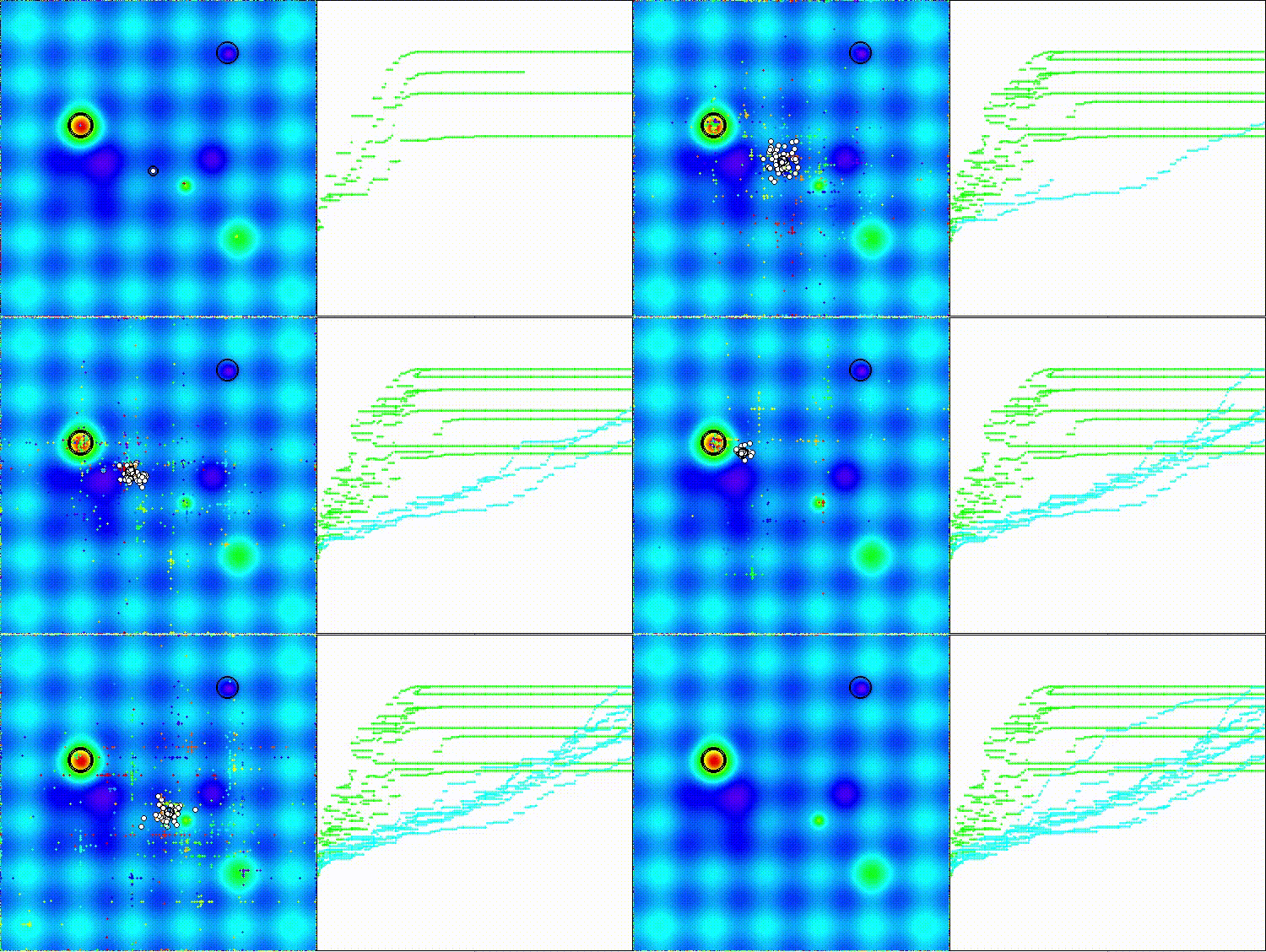
Hilly测试函数上的 CMA-ES
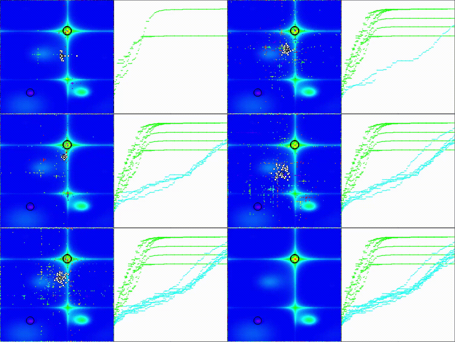
Forest 测试函数上的 CMA-ES
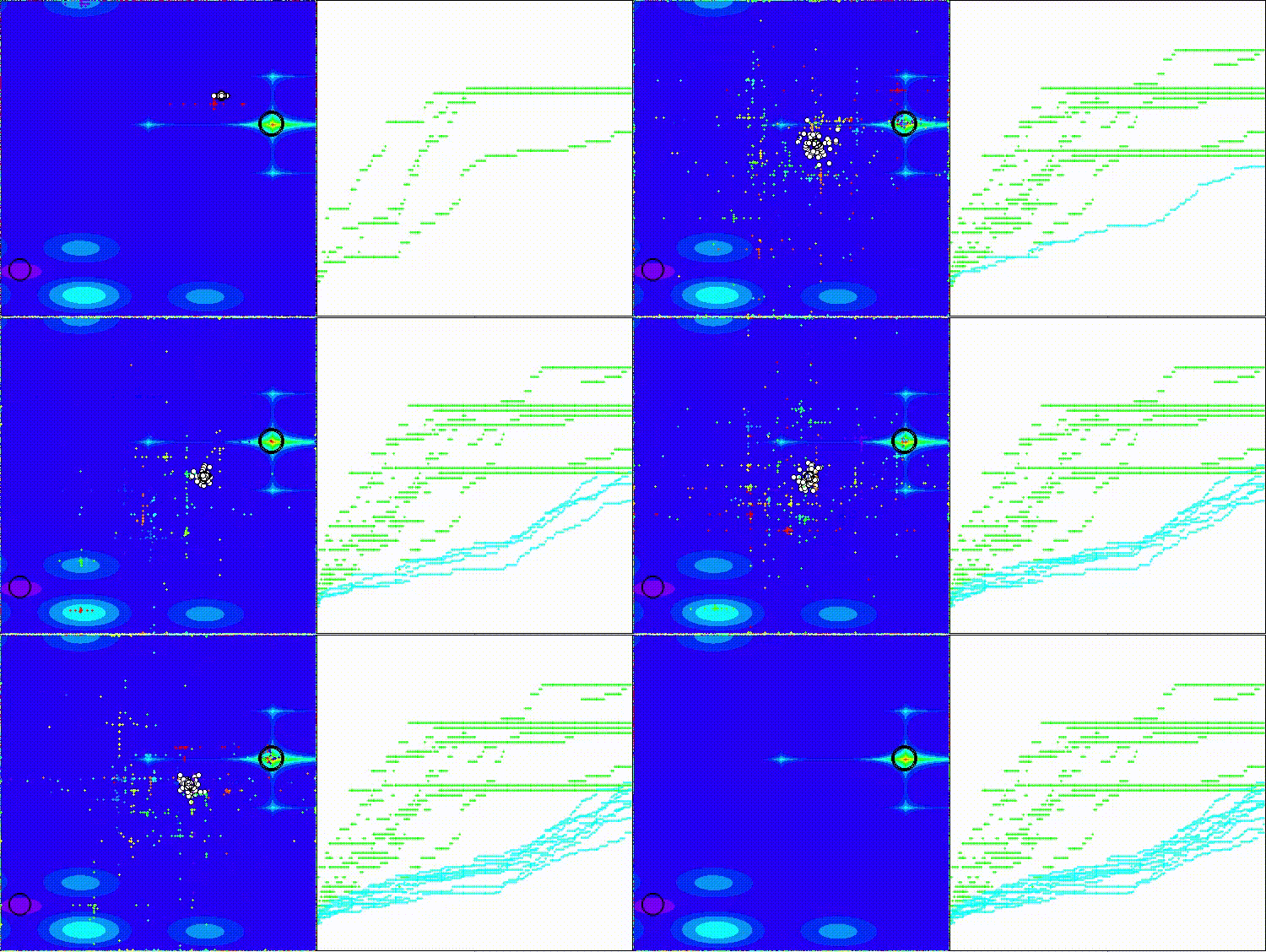
Megacity 测试函数上的 CMA-ES
根据结果,CMA-ES 算法在最强大的基于种群的优化算法排名中位列第 38。
# | AO | 描述 | Hilly | Hilly Final | Forest | Forest Final | Megacity (discrete) | Megacity Final | Final 结果 | % 的 最大限度 | ||||||
| 10 p(5 F) | 50 p(25 F) | 1000 p(500 F) | 10 p(5 F) | 50 p(25 F) | 1000 p(500 F) | 10 p(5 F) | 50 p(25 F) | 1000 p(500 F) | ||||||||
| 1 | ANS | 跨邻域搜索 | 0.94948 | 0.84776 | 0.43857 | 2.23581 | 1.00000 | 0.92334 | 0.39988 | 2.32323 | 0.70923 | 0.63477 | 0.23091 | 1.57491 | 6.134 | 68.15 |
| 2 | CLA | 密码锁算法(joo) | 0.95345 | 0.87107 | 0.37590 | 2.20042 | 0.98942 | 0.91709 | 0.31642 | 2.22294 | 0.79692 | 0.69385 | 0.19303 | 1.68380 | 6.107 | 67.86 |
| 3 | AMOm | 动物迁徙优化 M | 0.90358 | 0.84317 | 0.46284 | 2.20959 | 0.99001 | 0.92436 | 0.46598 | 2.38034 | 0.56769 | 0.59132 | 0.23773 | 1.39675 | 5.987 | 66.52 |
| 4 | (P+O)ES | (P+O)进化策略 | 0.92256 | 0.88101 | 0.40021 | 2.20379 | 0.97750 | 0.87490 | 0.31945 | 2.17185 | 0.67385 | 0.62985 | 0.18634 | 1.49003 | 5.866 | 65.17 |
| 5 | CTA | 彗尾算法(joo) | 0.95346 | 0.86319 | 0.27770 | 2.09435 | 0.99794 | 0.85740 | 0.33949 | 2.19484 | 0.88769 | 0.56431 | 0.10512 | 1.55712 | 5.846 | 64.96 |
| 6 | TETA | 时间演化旅行算法(joo) | 0.91362 | 0.82349 | 0.31990 | 2.05701 | 0.97096 | 0.89532 | 0.29324 | 2.15952 | 0.73462 | 0.68569 | 0.16021 | 1.58052 | 5.797 | 64.41 |
| 7 | SDSm | 随机扩散搜索 M | 0.93066 | 0.85445 | 0.39476 | 2.17988 | 0.99983 | 0.89244 | 0.19619 | 2.08846 | 0.72333 | 0.61100 | 0.10670 | 1.44103 | 5.709 | 63.44 |
| 8 | BOAm | 台球优化算法 M | 0.95757 | 0.82599 | 0.25235 | 2.03590 | 1.00000 | 0.90036 | 0.30502 | 2.20538 | 0.73538 | 0.52523 | 0.09563 | 1.35625 | 5.598 | 62.19 |
| 9 | AAm | 射箭算法 M | 0.91744 | 0.70876 | 0.42160 | 2.04780 | 0.92527 | 0.75802 | 0.35328 | 2.03657 | 0.67385 | 0.55200 | 0.23738 | 1.46323 | 5.548 | 61.64 |
| 10 | ESG | 社会群体的演化(joo) | 0.99906 | 0.79654 | 0.35056 | 2.14616 | 1.00000 | 0.82863 | 0.13102 | 1.95965 | 0.82333 | 0.55300 | 0.04725 | 1.42358 | 5.529 | 61.44 |
| 11 | SIA | 模拟各向同性退火(joo) | 0.95784 | 0.84264 | 0.41465 | 2.21513 | 0.98239 | 0.79586 | 0.20507 | 1.98332 | 0.68667 | 0.49300 | 0.09053 | 1.27020 | 5.469 | 60.76 |
| 12 | BBO | 基于生物地理学的优化 | 0.94912 | 0.69456 | 0.35031 | 1.99399 | 0.93820 | 0.67365 | 0.25682 | 1.86867 | 0.74615 | 0.48277 | 0.17369 | 1.40261 | 5.265 | 58.50 |
| 13 | ACS | 人工合作搜索 | 0.75547 | 0.74744 | 0.30407 | 1.80698 | 1.00000 | 0.88861 | 0.22413 | 2.11274 | 0.69077 | 0.48185 | 0.13322 | 1.30583 | 5.226 | 58.06 |
| 14 | DA | 辩证算法 | 0.86183 | 0.70033 | 0.33724 | 1.89940 | 0.98163 | 0.72772 | 0.28718 | 1.99653 | 0.70308 | 0.45292 | 0.16367 | 1.31967 | 5.216 | 57.95 |
| 15 | BHAm | 黑洞算法 M | 0.75236 | 0.76675 | 0.34583 | 1.86493 | 0.93593 | 0.80152 | 0.27177 | 2.00923 | 0.65077 | 0.51646 | 0.15472 | 1.32195 | 5.196 | 57.73 |
| 16 | ASO | 无政府社会优化 | 0.84872 | 0.74646 | 0.31465 | 1.90983 | 0.96148 | 0.79150 | 0.23803 | 1.99101 | 0.57077 | 0.54062 | 0.16614 | 1.27752 | 5.178 | 57.54 |
| 17 | RFO | 皇家同花顺优化(joo) | 0.83361 | 0.73742 | 0.34629 | 1.91733 | 0.89424 | 0.73824 | 0.24098 | 1.87346 | 0.63154 | 0.50292 | 0.16421 | 1.29867 | 5.089 | 56.55 |
| 18 | AOSm | 原子轨道搜索 M | 0.80232 | 0.70449 | 0.31021 | 1.81702 | 0.85660 | 0.69451 | 0.21996 | 1.77107 | 0.74615 | 0.52862 | 0.14358 | 1.41835 | 5.006 | 55.63 |
| 19 | TSEA | 龟壳进化算法(joo) | 0.96798 | 0.64480 | 0.29672 | 1.90949 | 0.99449 | 0.61981 | 0.22708 | 1.84139 | 0.69077 | 0.42646 | 0.13598 | 1.25322 | 5.004 | 55.60 |
| 20 | DE | 差异进化 | 0.95044 | 0.61674 | 0.30308 | 1.87026 | 0.95317 | 0.78896 | 0.16652 | 1.90865 | 0.78667 | 0.36033 | 0.02953 | 1.17653 | 4.955 | 55.06 |
| 21 | SRA | 成功的餐厅经营者算法(joo) | 0.96883 | 0.63455 | 0.29217 | 1.89555 | 0.94637 | 0.55506 | 0.19124 | 1.69267 | 0.74923 | 0.44031 | 0.12526 | 1.31480 | 4.903 | 54.48 |
| 22 | CRO | 化学反应优化 | 0.94629 | 0.66112 | 0.29853 | 1.90593 | 0.87906 | 0.58422 | 0.21146 | 1.67473 | 0.75846 | 0.42646 | 0.12686 | 1.31178 | 4.892 | 54.36 |
| 23 | BIO | 血统遗传优化(joo) | 0.81568 | 0.65336 | 0.30877 | 1.77781 | 0.89937 | 0.65319 | 0.21760 | 1.77016 | 0.67846 | 0.47631 | 0.13902 | 1.29378 | 4.842 | 53.80 |
| 24 | BSA | 鸟群算法 | 0.89306 | 0.64900 | 0.26250 | 1.80455 | 0.92420 | 0.71121 | 0.24939 | 1.88479 | 0.69385 | 0.32615 | 0.10012 | 1.12012 | 4.809 | 53.44 |
| 25 | HS | 和谐搜索 | 0.86509 | 0.68782 | 0.32527 | 1.87818 | 0.99999 | 0.68002 | 0.09590 | 1.77592 | 0.62000 | 0.42267 | 0.05458 | 1.09725 | 4.751 | 52.79 |
| 26 | SSG | 树苗播种和生长 | 0.77839 | 0.64925 | 0.39543 | 1.82308 | 0.85973 | 0.62467 | 0.17429 | 1.65869 | 0.64667 | 0.44133 | 0.10598 | 1.19398 | 4.676 | 51.95 |
| 27 | BCOm | 细菌趋化性优化 M | 0.75953 | 0.62268 | 0.31483 | 1.69704 | 0.89378 | 0.61339 | 0.22542 | 1.73259 | 0.65385 | 0.42092 | 0.14435 | 1.21912 | 4.649 | 51.65 |
| 28 | ABO | 非洲水牛优化 | 0.83337 | 0.62247 | 0.29964 | 1.75548 | 0.92170 | 0.58618 | 0.19723 | 1.70511 | 0.61000 | 0.43154 | 0.13225 | 1.17378 | 4.634 | 51.49 |
| 29 | (PO)ES | (PO)进化策略 | 0.79025 | 0.62647 | 0.42935 | 1.84606 | 0.87616 | 0.60943 | 0.19591 | 1.68151 | 0.59000 | 0.37933 | 0.11322 | 1.08255 | 4.610 | 51.22 |
| 30 | FBA | 基于分形的算法 | 0.79000 | 0.65134 | 0.28965 | 1.73099 | 0.87158 | 0.56823 | 0.18877 | 1.62858 | 0.61077 | 0.46062 | 0.12398 | 1.19537 | 4.555 | 50.61 |
| 31 | TSm | 禁忌搜索 M | 0.87795 | 0.61431 | 0.29104 | 1.78330 | 0.92885 | 0.51844 | 0.19054 | 1.63783 | 0.61077 | 0.38215 | 0.12157 | 1.11449 | 4.536 | 50.40 |
| 32 | BSO | 头脑风暴优化 | 0.93736 | 0.57616 | 0.29688 | 1.81041 | 0.93131 | 0.55866 | 0.23537 | 1.72534 | 0.55231 | 0.29077 | 0.11914 | 0.96222 | 4.498 | 49.98 |
| 33 | WOAm | 鲸鱼优化算法 M | 0.84521 | 0.56298 | 0.26263 | 1.67081 | 0.93100 | 0.52278 | 0.16365 | 1.61743 | 0.66308 | 0.41138 | 0.11357 | 1.18803 | 4.476 | 49.74 |
| 34 | AEFA | 人工电场算法 | 0.87700 | 0.61753 | 0.25235 | 1.74688 | 0.92729 | 0.72698 | 0.18064 | 1.83490 | 0.66615 | 0.11631 | 0.09508 | 0.87754 | 4.459 | 49.55 |
| 35 | AEO | 基于人工生态系统的优化算法 | 0.91380 | 0.46713 | 0.26470 | 1.64563 | 0.90223 | 0.43705 | 0.21400 | 1.55327 | 0.66154 | 0.30800 | 0.28563 | 1.25517 | 4.454 | 49.49 |
| 36 | CAm | 骆驼算法 M | 0.78684 | 0.56042 | 0.35133 | 1.69859 | 0.82772 | 0.56041 | 0.24336 | 1.63149 | 0.64846 | 0.33092 | 0.13418 | 1.11356 | 4.444 | 49.37 |
| 37 | ACOm | 蚁群优化 M | 0.88190 | 0.66127 | 0.30377 | 1.84693 | 0.85873 | 0.58680 | 0.15051 | 1.59604 | 0.59667 | 0.37333 | 0.02472 | 0.99472 | 4.438 | 49.31 |
| 38 | CMAES | 协方差矩阵自适应演化策略 | 0.76258 | 0.72089 | 0.00000 | 1.48347 | 0.82056 | 0.79616 | 0.00000 | 1.61672 | 0.75846 | 0.49077 | 0.00000 | 1.24923 | 4.349 | 48.33 |
| 39 | BFO-GA | 细菌觅食优化 - ga | 0.89150 | 0.55111 | 0.31529 | 1.75790 | 0.96982 | 0.39612 | 0.06305 | 1.42899 | 0.72667 | 0.27500 | 0.03525 | 1.03692 | 4.224 | 46.93 |
| 40 | SOA | 简单优化算法 | 0.91520 | 0.46976 | 0.27089 | 1.65585 | 0.89675 | 0.37401 | 0.16984 | 1.44060 | 0.69538 | 0.28031 | 0.10852 | 1.08422 | 4.181 | 46.45 |
| 41 | ABHA | 人工蜂巢算法 | 0.84131 | 0.54227 | 0.26304 | 1.64663 | 0.87858 | 0.47779 | 0.17181 | 1.52818 | 0.50923 | 0.33877 | 0.10397 | 0.95197 | 4.127 | 45.85 |
| 42 | ACMO | 大气云模型优化 | 0.90321 | 0.48546 | 0.30403 | 1.69270 | 0.80268 | 0.37857 | 0.19178 | 1.37303 | 0.62308 | 0.24400 | 0.10795 | 0.97503 | 4.041 | 44.90 |
| 43 | ADAMm | 自适应矩估计 M | 0.88635 | 0.44766 | 0.26613 | 1.60014 | 0.84497 | 0.38493 | 0.16889 | 1.39880 | 0.66154 | 0.27046 | 0.10594 | 1.03794 | 4.037 | 44.85 |
| 44 | CGO | 混沌游戏优化 | 0.57256 | 0.37158 | 0.32018 | 1.26432 | 0.61176 | 0.61931 | 0.62161 | 1.85267 | 0.37538 | 0.21923 | 0.19028 | 0.78490 | 3.902 | 43.35 |
| 45 | CROm | 珊瑚礁优化 M | 0.78512 | 0.46032 | 0.25958 | 1.50502 | 0.86688 | 0.35297 | 0.16267 | 1.38252 | 0.63231 | 0.26738 | 0.10734 | 1.00703 | 3.895 | 43.27 |
| RW | 随机游走 | 0.48754 | 0.32159 | 0.25781 | 1.06694 | 0.37554 | 0.21944 | 0.15877 | 0.75375 | 0.27969 | 0.14917 | 0.09847 | 0.52734 | 2.348 | 26.09 | |
总结
CMA-ES 能够根据目标函数的局部几何特性调整搜索策略,这一能力使其在处理具有未知结构的复杂、病态问题时几乎不可或缺。幂律分布的重尾使得该算法能够进行“长跳跃”,这对于逃离局部最优解至关重要。该算法的计算复杂度为 O(n²) 内存和 O(n³) 时间,严重限制了其适用性。对于高维问题(n > 100),资源投入强度与所获得的收益不成比例。多维函数的运行时间增长如此之快,以至于对于较大的 n 值,该算法几乎无法应用。
CMA-ES 适用于噪声函数,能够处理不连续的目标函数,在多极值景观上表现有效,而这种多样性的秘诀在于该算法的基本理念:它不对函数结构做出假设,而是对其进行细致探索,并根据积累的经验调整其搜索策略。CMA-ES 重新定义了进化计算中的一类方法,它表明生物启发式算法可以具有严格的数学基础,并且算法适应不仅仅是参数调整,而是学习问题结构的基本原则。
该算法对于中等规模的问题而言非常出色,它是一款专业工具,在其细分领域中看起来是一个值得考虑的替代方案。该算法兼具数学上的优雅与实际中的高效,但由于其计算上的局限性,使用时需谨慎。在这种情况下,MQL5 语言开发人员最近引入了快速的 MQL5 矩阵操作来计算矩阵;在此算法实现中,使用了传统的顺序计算。
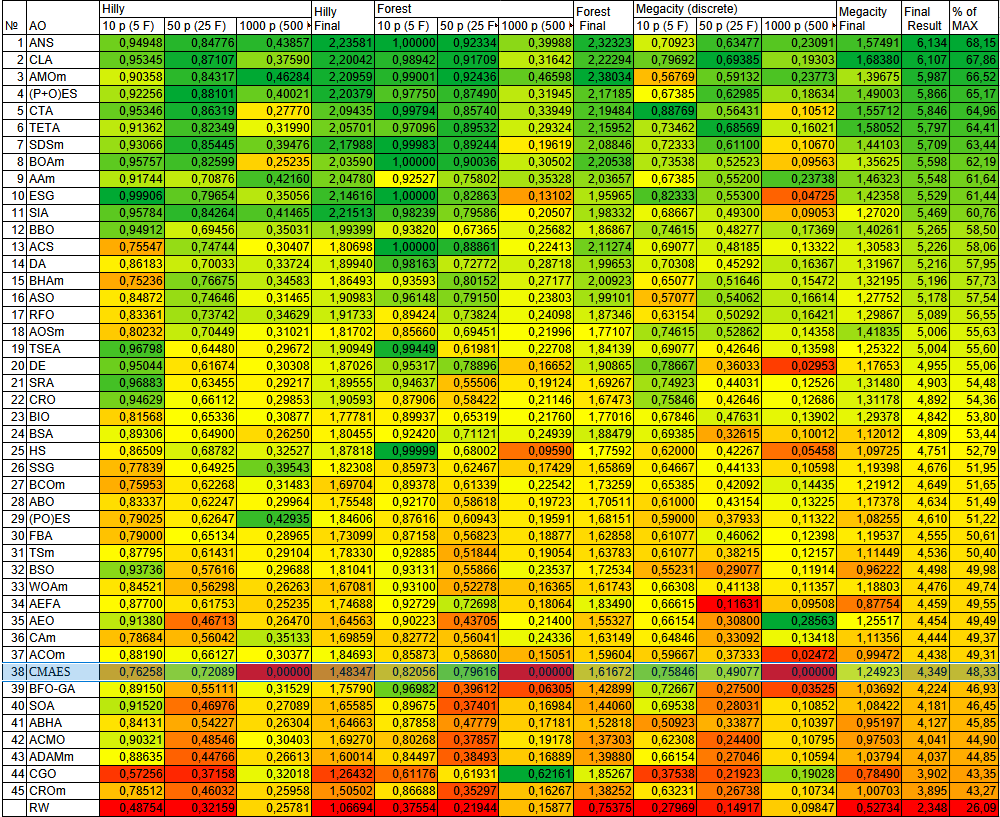
图2.根据相应测试的算法颜色分级
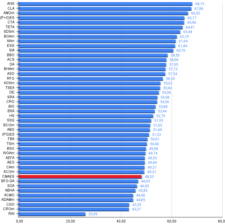
图 3.算法测试结果直方图(范围从 0 到 100,越高越好,其中 100 是可能的最大理论结果,存档中有一个用于计算评级表的脚本)
CMAES 的优点和缺点:
优点:
- 对中等维度的函数具有良好的收敛性。
缺点:
- 低维函数的结果分散。
- 大尺度函数的关键资源密集度。
这篇文章附有一个归档,其中包含当前版本的算法代码。文章作者不对规范算法描述的绝对准确性负责。为提高搜索能力,已对其中多项功能进行了修改。文章中提出的结论和判断都是基于实验结果。
本文中用到的程序
| # | 名称 | 类型 | 描述 |
|---|---|---|---|
| 1 | #C_AO.mqh | 包含文件 | 种群优化算法的父类 |
| 2 | #C_AO_enum.mqh | 包含文件 | 种群优化算法的枚举 |
| 3 | TestFunctions.mqh | 包含文件 | 测试函数库 |
| 4 | TestStandFunctions.mqh | 包含文件 | 测试平台函数库 |
| 5 | Utilities.mqh | 包含文件 | 辅助函数库 |
| 6 | CalculationTestResults.mqh | 包含文件 | 用于计算比较表中结果的脚本 |
| 7 | Testing AOs.mq5 | 脚本 | 所有种群优化算法的统一测试平台 |
| 8 | Simple use of population optimization algorithms.mq5 | 脚本 | 使用不带可视化的种群优化算法的简单示例 |
| 9 | Test_AO_CMAES.mq5 | 脚本 | CMAES 测试平台 |
本文由MetaQuotes Ltd译自俄文
原文地址: https://www.mql5.com/ru/articles/18227
注意: MetaQuotes Ltd.将保留所有关于这些材料的权利。全部或部分复制或者转载这些材料将被禁止。
本文由网站的一位用户撰写,反映了他们的个人观点。MetaQuotes Ltd 不对所提供信息的准确性负责,也不对因使用所述解决方案、策略或建议而产生的任何后果负责。

 MQL5中的自优化智能交易系统(第十部分):矩阵分解

 在 MQL5 中实现保本机制(第 2 部分):基于 ATR 和风险回报比的保本机制

