Persistent Homology in MQL5: The Reduction Algorithm and the Persistence Diagram

Contents

1. Introduction: From Boundary Matrix to Diagram
2. A Persistence Diagram on a Chart
3. Homology: What the Diagram Counts
4. The Reduction Algorithm
5. Implementation: CTDAReduction
6. Essential Features and a Truncation Artifact
7. The Diagram: SPersistencePair and CTDADiagram
8. The CTDA Facade
9. Verification Against Ripser
10. What's Next
11. Conclusion

Introduction: From Boundary Matrix to Diagram

In the previous article we built two classes. The Vietoris-Rips filtration enumerated every vertex, edge, and triangle, sorted by the scale at which it enters the complex. The boundary matrix recorded, for each simplex, the lower-dimensional simplices that form its border. We ended with a sorted list of simplices and a sparse matrix over Z/2.

That matrix holds the answer, but not in readable form. The loops and connected components are encoded in its column relationships, not stated outright. Extracting them is the job of one algorithm: the standard column reduction. It is the computational heart of persistent homology, and it is what this article implements.

The output is a persistence diagram. Each entry is a birth-death pair: a topological feature, its homology dimension, the scale at which it appeared, and the scale at which it vanished. Long-lived pairs are real structure. Short-lived pairs are noise. This is the payoff the first two articles were building toward.

This article introduces three classes. CTDAReduction runs the reduction. CTDADiagram stores the resulting pairs and answers questions about them. CTDA is a facade that runs the whole six-step pipeline in one call. By the end, you can pass a price window to a single Compute call. It returns a persistence diagram whose birth and death values match an independent reference to six decimal places. The article closes with that verification: a bit-for-bit comparison against Ripser.

A Persistence Diagram on a Chart

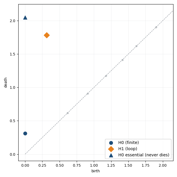
Fig. 1. The persistence diagram of a unit circle sampled at 20 points. Nineteen H0 component bars die at 0.3129, one H0 component never dies, and a single H1 loop is born at 0.3129 and dies at 1.7820.

The figure above is the finished product. It is the persistence diagram of a circle sampled at 20 points, computed end-to-end by this library. The horizontal axis is birth, the vertical axis is death, and every point is one topological feature.

Read it in two parts. Near the bottom left, a single blue marker holds nineteen H0 bars: nineteen of the twenty points merge into their neighbors at scale 0.3129. The blue triangle at the top is the one connected component that never dies. The orange diamond high above the diagonal is the prize: one H1 loop, born when the ring closes at 0.3129 and filled in at 1.7820. One circle, one loop. The diagram says so with one point.

That is what this article delivers. The rest explains how the reduction produces it, and how we know the numbers are right.

Homology: What the Diagram Counts

Persistent homology counts holes, organized by dimension. The notation is H0, H1, H2, and each dimension counts a different kind of feature.

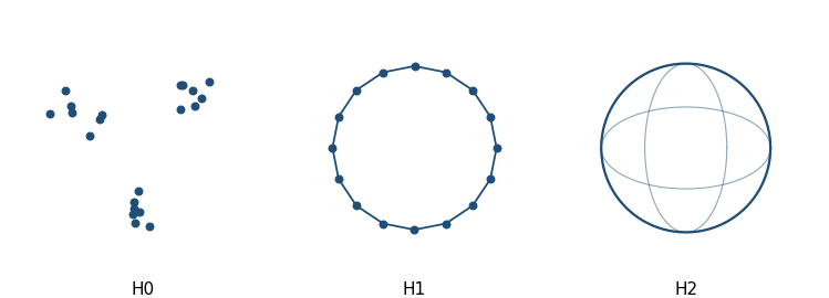
Fig. 2. Persistent homology counts connected components (H0), loops (H1), and enclosed voids (H2).

H0 counts connected components. At a tiny scale every point is its own component. As the scale grows, points merge. Each merge kills one H0 feature. The number of H0 features alive at a given scale is how many separate pieces the cloud has at that scale.

H1 counts loops. A loop is a closed ring of edges with an empty interior, like the middle panel of the previous article. It is born when the ring closes and dies when triangles fill the interior. A loop that stays open across a wide range of scales is a real cycle in the data.

H2 counts voids. A void is an enclosed cavity, the inside of a hollow sphere. This library builds simplices up to triangles, so it detects H0 and H1 reliably. Genuine H2 detection needs tetrahedra, which we do not build. A later section explains how the library handles the H2 artifacts that the truncation creates.

Every feature has a birth and a death, measured in the same scale parameter epsilon that drives the filtration. The persistence of a feature is death minus birth. A feature that never dies within the filtration is called essential and carries an infinite death value.

On the birth-death plane of Figure 1, persistence is the vertical distance from the diagonal. Points near the diagonal are born and die at almost the same scale, so they are short-lived noise. Points far above the diagonal survive across many scales, and those are the features worth attention. Reading a persistence diagram is mostly a matter of ignoring the diagonal and looking at what floats above it. The single orange diamond of the circle is the whole point of the method: one number that says "there is one loop here, and it is real".

The Reduction Algorithm

The boundary matrix has one column per simplex, ordered by filtration. Each column lists the faces of its simplex as row indices, sorted ascending. The pivot of a column is its lowest face, which is its last entry because the column is sorted. The reduction makes every pivot unique.

The procedure is short. Process the columns left to right. For each column, look at its pivot. If an earlier column already owns that pivot row, add the earlier column to this one. Over Z/2, adding two columns is the symmetric difference of their face sets: shared faces cancel, the rest survive. The addition changes the pivot. Repeat until either the pivot is new, or the column becomes empty.

A new pivot means a death. The column's simplex fills in a feature that an earlier simplex created. The pair is recorded: birth at the pivot simplex, death at the current simplex. An empty column means a birth. The simplex created a feature that nothing has killed yet. These unpaired creators become the essential features.

Two design points make this fast. The columns are kept sorted, so reading a pivot is a single array access at the end. A pivot table maps each occupied pivot row to the column that owns it, so finding the column to add is one lookup, not a scan. The cost is dominated by the symmetric-difference additions, and the triangle count from the previous article is why the reduction is the most expensive stage of the pipeline.

It helps to see the reduction as Gaussian elimination over the two-element field. Each column addition is a row operation, and the end state is a matrix where no two columns share a pivot. A foundational result of persistent homology is that the pairing does not depend on the order of column additions. Regardless of the addition sequence, the algorithm produces the same set of birth-death pairs. That invariance is what lets us trust a single left-to-right pass, and it is also what makes the comparison against an independent implementation meaningful.

Implementation: CTDAReduction

The single most-used operation is the column addition over Z/2. It merges two sorted face lists and drops any face that appears in both.

//+------------------------------------------------------------------+
//| Symmetric difference of two sorted ascending int arrays          |
//+------------------------------------------------------------------+
void CTDAReduction::XorColumns(const int &a[], const int &b[], int &out[]) const
  {
   int na = ArraySize(a);
   int nb = ArraySize(b);
   ArrayResize(out, na + nb);
   int i = 0, j = 0, k = 0;
   while(i < na && j < nb)
     {
      if(a[i] < b[j])      { out[k++] = a[i++]; }
      else if(a[i] > b[j]) { out[k++] = b[j++]; }
      else                  { i++; j++; }   // equal entries cancel under Z/2
     }
   while(i < na) out[k++] = a[i++];
   while(j < nb) out[k++] = b[j++];
   ArrayResize(out, k);
  }

The routine walks both arrays in lockstep, like a sorted-list merge. When the two fronts differ, the smaller index is copied out. When they are equal, both are skipped: a face present in both columns cancels modulo 2. Leftover entries from either list are appended. The result is the symmetric difference, still sorted, ready to be a column again.

The main loop drives the reduction. For each column it reads the pivot, and either adds the stored owner of that pivot or claims the pivot as new.

   //--- main reduction loop
   for(int j = 0; j < numCols; j++)
     {
      boundary.GetColumn(j, workCol);
      int currentSize = ArraySize(workCol);

      while(currentSize > 0)
        {
         int p = workCol[currentSize - 1];   // pivot = last (largest) entry

         if(m_pivotCol[p] >= 0)
           {
            //--- XOR with the stored reduced column for pivot row p
            int start = m_reducedStart[p];
            int sz    = m_reducedSize[p];
            ArrayResize(storedCol, sz);
            for(int k = 0; k < sz; k++)
               storedCol[k] = m_reducedEntries[start + k];

            XorColumns(workCol, storedCol, xorOut);

            int newSize = ArraySize(xorOut);
            ArrayResize(workCol, newSize);
            for(int k = 0; k < newSize; k++)
               workCol[k] = xorOut[k];
            currentSize = newSize;
           }
         else
           {
            //--- new pivot found at row p -> record persistence pair
            m_pivotCol[p] = j;
            StoreReducedColumn(p, workCol);

            SSimplex sBirth, sDeath;
            rips.Get(p, sBirth);
            rips.Get(j, sDeath);

            // emit pair only if persistence > 0 (sometimes filtration ties give 0-length)
            // we keep zero-persistence pairs too - they are valid topological events
            diagram.Add(sBirth.filtration, sDeath.filtration, sBirth.dim, p, j);
            break;
           }
        }

      if(currentSize == 0)
         m_isCreator[j] = true;
     }

The inner while loop is the reduction. It reads the pivot p as the last entry of the working column. If m_pivotCol[p] already holds an owner, the stored reduced column for that pivot is fetched and added with XorColumns, which shrinks or shifts the working column and changes its pivot. If the pivot row is free, the column has found a new pivot. The library records the birth-death pair from the two simplices, stores the reduced column under its pivot for future additions, and breaks. A column that reduces all the way to empty created a feature, so it is flagged as a creator.

The birth-death pair comes straight from the filtration values. The simplex at the pivot row is the creator, so its filtration is the birth. The current simplex is the killer, so its filtration is the death. The library keeps pairs even when birth equals death, because a zero-length bar is still a valid event. Those are filtered out later when it matters.

A Reduction by Hand

The four-point loop from the previous article makes the algorithm concrete. Take four points at the corners of a square, joined by four side edges, with the diagonals too long to enter. The simplices, in filtration order, are four vertices and then four edges:

0: v0 1: v1 2: v2 3: v3 4: e01 5: e12 6: e23 7: e30

The four vertex columns are empty, so every vertex is a creator. Four connected components are born at scale zero. The first three edges each find a free pivot and pair off at once, recording three component deaths as the points merge into one piece:

e01 pivot v1 gives (v1, e01), e12 pivot v2 gives (v2, e12), e23 pivot v3 gives (v3, e23)

The fourth edge is where the loop appears. Column e30 starts as the face set {v0, v3}, and its pivot v3 is already owned by e23. The reduction now adds columns until the pivot is new or the column empties:

Step	Working column	Pivot	Action
e30 start	{v0, v3}	v3	pivot owned by e23, add it
+ e23 {v2, v3}	{v0, v2}	v2	pivot owned by e12, add it
+ e12 {v1, v2}	{v0, v1}	v1	pivot owned by e01, add it
+ e01 {v0, v1}	{ } empty	none	column empties: a loop is born

Column e30 reduces to nothing. An empty column is the signature of a creator: the fourth edge closes a cycle that no earlier simplex accounts for. There is no triangle to fill the square, so nothing ever kills this loop, and it is emitted as an essential H1 feature. The final diagram has one connected component, three finite H0 bars, and one essential H1 loop. That is exactly the topology of a square outline: one piece, one hole.

Essential Features and a Truncation Artifact

After every column is processed, the creators that were never used as a pivot are the essential features. They never die in the filtration, so they carry an infinite death value. The H0 essential is the single connected component that survives to the end. An H1 essential is a loop that the filtration never fills.

There is one honest complication. This library stops at triangles, so the top dimension is 2. A triangle that creates an H2 feature can only be killed by a tetrahedron, and there are no tetrahedra. Every such triangle would therefore be reported as an essential H2 feature, even though it is not a real void. These are artifacts of stopping the filtration early, not genuine cavities.

   //--- emit essential features
   //    A creator simplex at the maximum built dimension can never be killed,
   //    so when maxDim = 2 every triangle that does not kill an H1 becomes
   //    a spurious "essential H2" feature (filtration-truncation artifact).
   //    For clean H0 + H1 analysis we suppress these by default;
   //    H0 and H1 essentials are always emitted.
   int ripsMaxDim = rips.MaxDim();
   for(int j = 0; j < numCols; j++)
     {
      if(!m_isCreator[j])      continue;
      if(m_pivotCol[j] >= 0)   continue;

      SSimplex s;
      rips.Get(j, s);

      //--- only the top-dim essentials when maxDim = 2 are dropped;
      //    in maxDim = 1 mode the H1 essentials are the real loops.
      if(!m_emitTopDimEssentials && ripsMaxDim >= 2 && s.dim == ripsMaxDim)
         continue;

      diagram.Add(s.filtration, TDA_INF, s.dim, j, -1);
     }

The loop emits an infinite bar for each unpaired creator, with one guard. When the maximum built dimension is 2, a creator at dimension 2 is suppressed by default, because it is a truncation artifact rather than a real void. The H0 and H1 essentials are always emitted, since those are real. The behavior is configurable: a call to SetEmitTopDimEssentials(true) (not shown here) restores the raw output for a caller that wants it. For ordinary H0 and H1 analysis the default keeps the diagram clean.

The Diagram: SPersistencePair and CTDADiagram

Each feature is one struct. It records the birth and death scales, the homology dimension, and the two simplices involved.

//+------------------------------------------------------------------+
//| SPersistencePair - one topological feature (birth, death, dim)   |
//|                                                                  |
//|  A persistent feature is born at filtration value 'birth' (when  |
//|  the simplex that creates it enters the complex) and dies at     |
//|  'death' (when a higher-dim simplex fills it in). Features that  |
//|  never die in the filtration carry death = TDA_INF.              |
//+------------------------------------------------------------------+
struct SPersistencePair
  {
   double   birth;          // filtration value when feature appears
   double   death;          // filtration value when feature dies (TDA_INF if alive)
   int      dim;            // homological dimension (0 = component, 1 = loop, 2 = void)
   int      birthSimplex;   // simplex index that created this feature
   int      deathSimplex;   // simplex index that killed it (-1 if alive)

   double   Persistence() const
     {
      return (death >= TDA_INF) ? TDA_INF : (death - birth);
     }

   bool     IsInfinite() const
     {
      return (death >= TDA_INF);
     }

   void     Reset()
     {
      birth        = 0.0;
      death        = 0.0;
      dim          = 0;
      birthSimplex = -1;
      deathSimplex = -1;
     }
  };

The two helper methods carry the meaning. Persistence is death minus birth, with the infinite case handled explicitly. IsInfinite marks essential features, which use TDA_INF (defined as DBL_MAX) as a death sentinel. The dimension field tells H0 from H1 from H2.

The CTDADiagram class collects these pairs and answers questions about them: how many pairs in a dimension, the total and maximum persistence, and the Betti number at any scale. The Betti number is the count of features alive at a chosen epsilon, which is exactly what the persistence diagram encodes.

//+------------------------------------------------------------------+
//| Number of features alive at a given filtration value (Betti)     |
//+------------------------------------------------------------------+
int CTDADiagram::BettiNumber(int dim, double epsilon) const
  {
   int c = 0;
   for(int i = 0; i < m_count; i++)
     {
      if(m_pairs[i].dim != dim) continue;
      if(m_pairs[i].birth > epsilon) continue;          // not yet born
      if(!m_pairs[i].IsInfinite()
         && m_pairs[i].death <= epsilon) continue;       // already dead
      c++;
     }
   return c;
  }

A feature is alive at epsilon if it was born at or before epsilon and has not yet died. The method skips features not yet born, skips finite features that have already died, and counts the rest. Sweeping epsilon from zero upward turns the diagram into a Betti curve, the count of components or loops as a function of scale.

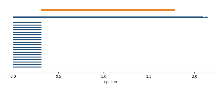
Fig. 3. The same diagram as a barcode. Each bar runs from birth to death. The single long H1 bar is the one loop of the circle.

The barcode above is the same information in a different view. Each feature is a horizontal bar from its birth to its death. The nineteen short H0 bars end at 0.3129. The H0 essential bar runs off the right edge. The single long H1 bar is the loop. One long bar in H1 means one loop, read at a glance.

The CTDA Facade

The six stages, point cloud, distance matrix, filtration, boundary, reduction, and diagram, always run in the same order. The CTDA facade wires them together so a caller never touches the internals.

//+------------------------------------------------------------------+
//| Full pipeline: series to persistence diagram                     |
//+------------------------------------------------------------------+
bool CTDA::Compute(const double &series[], int N)
  {
   m_computed = false;
   m_diagram.Clear();

   if(N < 4)
     {
      Print("CTDA::Compute - series too short (min 4 bars)");
      return false;
     }

   //--- 1. Embed series into point cloud
   if(!m_cloud.Build(series, N, m_embDim, m_delay))
      return false;

   //--- 2. Compute full pairwise distance matrix
   if(!m_distance.Build(m_cloud, m_norm))
      return false;

   //--- 3. Determine maxEpsilon (auto vs fixed)
   double maxEps = m_maxEpsilon;
   if(m_autoEpsilon)
      maxEps = m_distance.MaxDistance() * m_maxEpsilonFrac;
   if(maxEps <= 0.0)
     {
      Print("CTDA::Compute - invalid maxEpsilon (<= 0)");
      return false;
     }
   m_maxEpsilon = maxEps;

   //--- 4. Build Vietoris-Rips filtration
   if(!m_rips.Build(m_distance, maxEps, m_maxDim))
      return false;

   //--- 5. Build boundary matrix
   if(!m_boundary.Build(m_rips))
      return false;

   //--- 6. Reduce boundary -> persistence pairs
   if(!m_reduction.Compute(m_rips, m_boundary, m_diagram))
      return false;

   m_computed = true;
   return true;
  }

Compute runs the pipeline end-to-end and stops at the first failure. It embeds the series with the Takens method from the first article, builds the pairwise distance matrix, picks the VR cutoff (a fraction of the cloud diameter by default), builds the filtration and boundary matrix from the second article, and reduces. When it returns true, the diagram is ready to query. From the caller's side the entire topological machinery is one method call.

A short script shows the whole interface.

#include <TDA/TDA.mqh>

void OnStart()
  {
   double close[];
   if(CopyClose(_Symbol, _Period, 0, 120, close) != 120)
      return;

   CTDA tda;
   tda.SetEmbedding(3, 1);          // dimension d = 3, delay tau = 1
   tda.SetMaxEpsilonAuto(1.0);      // VR cutoff = full cloud diameter
   tda.SetMaxDim(2);                // compute H0 and H1

   if(tda.Compute(close, 120))
     {
      tda.PrintSummary();
      double h1 = tda.PersistenceEntropy(1);
      PrintFormat("H1 persistence entropy = %.4f", h1);
     }
  }

The caller sets the embedding dimension and delay, chooses an automatic VR cutoff, and asks for H0 and H1. After Compute returns, the diagram and every derived metric are available. The persistence entropy used by the indicator in the next article is one such metric, computed directly from the finite bars in a dimension.

Verification Against Ripser

A topology library is only useful if its numbers are correct. The persistence diagrams produced by this library have been validated against the Ripser reference implementation to within 10^-6 on seven independent test cases: six synthetic geometries plus a live 80-bar market window processed end-to-end through the full Takens-embedding pipeline.

The verification runs at three levels of increasing rigor.

Level	Script	What it checks
1	TDA_Test_KnownTopology.mq5	Behavioral signatures: periodic, chaotic, trivial
2	TDA_Test_GroundTruth.mq5	Exact birth/death against analytical predictions on 7 clouds
3	TDA_Export_*.mq5 + tda_crosscheck.py	Bit-for-bit agreement with Ripser, including live market data

Level 2 checks exact values against hand-derived geometry. On the unit circle with N=20 points, the library reports the H1 loop birth at 0.312869, matching the analytical chord length 2 sin(pi/20) to six decimal places. The loop then dies at 1.782013, for a persistence of 1.469144, the single dominant H1 feature of the circle. Across seven geometric cases the suite runs 31 independent checks, and all 31 pass.

Level 3 is the strict one. The same clouds are exported to CSV, Python runs Ripser on them, and the two diagrams are compared bar by bar.

Case	Points	MQL5 pairs	Ripser bars	Result
unit circle, N=20	20	191	21	match
unit circle, N=50	50	1226	51	match
two clusters	10	46	11	match
two disjoint circles	20	191	22	match
random scatter	30	436	31	match
sine embedding	75	2776	21	match
live market window	78	3004	91	match

The pair counts differ by design. The library keeps every pair, including the zero-length bars where birth equals death. Ripser discards those by default. After the zero-persistence bars are filtered, the non-trivial bars agree to within 10^-6 in every case. The MQL5 column reports the raw count, the Ripser column the filtered count, and the right-hand result is the comparison after filtering.

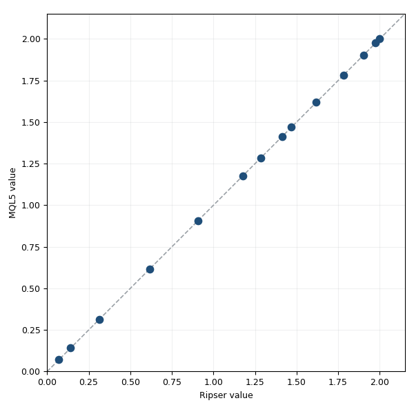
Fig. 4. Each persistence value from the library plotted against the Ripser value for the same bar. All points lie on the diagonal, the visual form of agreement to within 10^-6 across the seven cross-check cases.

The last case is not a synthetic geometry. It is a live 80-bar window taken straight from a chart (XAU/USD on the one-minute timeframe in this run), embedded with the same library, and exported as a CSV. Python loads that CSV, runs Ripser, and the 91 non-trivial bars agree. The pipeline that will drive the indicator in the next article produces diagrams that match an independent reference on real market data.

This agreement rules out the key failure modes. Any off-by-one error in boundary faces, or any sign, ordering, pivot-rule, or filtration-sort error, would shift at least one birth or death value from its correct position. Across seven clouds, from a clean circle to a noisy live window, every non-trivial bar lands where the reference puts it. The pipeline is internally consistent and matches results computed by an independent implementation in a different language.

A note on claims. The library is not faster than Ripser, and the word "exact" is reserved for the filtered comparison: agreement to within 10^-6 after zero-persistence bars are removed. That is the honest statement, and it is enough.

What's Next

The library is verified. It turns a price window into a persistence diagram whose numbers match an independent reference. The final article puts that diagram to work on a live chart.

• Persistence entropy: a single number summarizing the spread of bar lengths in a dimension.
• H0 entropy as market fragmentation, H1 entropy as cyclical complexity.
• The PersistenceEntropy_Indicator, its sliding-window design, and the guards that keep it responsive.
• Live regime examples and a sketch of reading CTDA output from an EA.

Conclusion

This article completed the engine. It reduced the boundary matrix into a persistence diagram and verified the result.

• CTDAReduction runs the standard Z/2 column reduction, pairing creators with killers and emitting the rest as essential features, with top-dimension artifacts suppressed by default.
• CTDADiagram and SPersistencePair store the birth-death pairs and answer questions: counts per dimension, total and maximum persistence, Betti numbers, and persistence entropy.
• CTDA wraps the six-stage pipeline into one Compute call.

You can now run the whole pipeline yourself. One CTDA::Compute call on a price window returns a persistence diagram, and CTDADiagram answers every question about it: counts per dimension, total and maximum persistence, Betti numbers, and persistence entropy. The numbers are not asserted, they are checked. Thirty-one of thirty-one ground-truth checks pass, and the diagrams match Ripser to within 10^-6 on seven cases, including live market data. The next article turns this verified pipeline into a market regime indicator.

The files attached to this article are also available on Algo Forge.

#	Filename	Type	Description
1	TDAPointCloud.mqh	Header	Takens embedding (from Article 1)
2	TDADistance.mqh	Header	Pairwise distance matrix (from Article 1)
3	TDARips.mqh	Header	Vietoris-Rips filtration (from Article 2)
4	TDABoundary.mqh	Header	Boundary matrix over Z/2 (from Article 2)
5	TDAReduction.mqh	Header	Column reduction to persistence pairs (this article)
6	TDADiagram.mqh	Header	Persistence diagram and analytics (this article)
7	TDA.mqh	Header	CTDA facade, full pipeline (this article)
8	TDA_Facade_Demo.mq5	Script	Runnable facade demo: one Compute call to a persistence diagram
9	TDA_Test_KnownTopology.mq5	Script	Level-1 behavioral signature checks
10	TDA_Test_GroundTruth.mq5	Script	Level-2 ground-truth checks (31/31)
11	TDA_Export_For_Crosscheck.mq5	Script	Exports synthetic clouds for the Ripser cross-check
12	TDA_Export_LiveMarket.mq5	Script	Exports a live market window for the cross-check
13	tda_crosscheck.py	Python	Runs Ripser and compares to the MQL5 output