Ollivier-Ricci Curvature: Reading the Shape of a Correlation Network, Not Its Level

Contents

• Introduction
• What the gauge reads on a real market
• Curvature on a graph, in one formula
• The transport problem, solved exactly
• Twenty-six symbols on one clock
• The two decisions that decide whether the number means anything
• The nulls, including the one that is empty
• What real markets read
• The indicator, and the expert
• Verification
• Conclusion

Introduction

Every correlation dashboard on this site answers the same question: how strongly are these instruments moving together right now? That number is useful, but it is a level, and a level cannot say whether the market still has any internal structure left. A market where metals move with metals, indices with indices, and the yen moves against everything is different from one where all twenty-six instruments collapse onto a single driver. Yet both can report the same average correlation.

Sandhu, Georgiou and Tannenbaum made the case in 2016 that the missing quantity is a geometric one. Build a network whose nodes are the instruments and whose edge lengths come from their correlations, then ask a question from Riemannian geometry: is this network locally curved? On a positively curved edge the endpoints share most of their neighborhoods, so there are many ways round and no connection is load bearing. On a negatively curved edge there is one way across, and cutting it splits the market in two. Curvature is a statement about shape that barely moves with the correlation level, which is the property no correlation average can have.

This article builds that measurement in MQL5 from nothing. The definition used is Ollivier's:

kappa(x, y) = 1 - W1(m_x, m_y) / d(x, y)

where d is the distance between two instruments, m_x is a probability measure spread over x's neighborhood, and W1 is the optimal transport cost of turning one of those measures into the other. Everything in the library is arithmetic around that one quantity, so the transport solver is the foundation and is solved exactly.

One warning belongs at the top, because it shapes every design choice below. The raw curvature value has no standalone interpretation: it sits on a compressed scale whose structureless reference depends only on the basket size, so a reading of 0.47 is neither high nor low on its own. That is why the library never ships a number without a null beside it, and why this article treats the point as a result rather than a caveat.

What the gauge reads on a real market

Here is the tool doing its job before the machinery is explained: the opening of ORC_Scan_Market.mq5 on a twenty-six symbol basket of majors, crosses, metals, energy, indices and crypto, daily bars, a rolling correlation window of 120 bars, stepping five bars at a time from January 2020 to August 2026.

[ORC] ==== market scan start ====
[ORC] == 1. the basket =================================
[ORC] 26 of 26 symbols, 2041 aligned bars from 2019.07.16 to 2026.08.17; start date set by US30m
[ORC] requested 26, kept 26, dropped 0
[ORC] weakest kept coverage: JP225m at 97.6%
[ORC] structureless pole for 26 symbols: 0.520000
[ORC] == 2. the rolling reading ========================
[ORC] 385 readings, 2020.01.07 to 2026.08.17, step 5 bars
[ORC] kappa  min 0.459595  mean 0.475096  max 0.483299  sd 0.005289
[ORC] gap from the pole  min 0.036701  mean 0.044904  max 0.060405
[ORC] avg |rho| ranged 0.251 to 0.451
[ORC] cost 137.2 ms per window, 0 refused
[ORC] == 2b. curvature versus average correlation =======
[ORC] kappa vs avg|rho| over 385 windows: Pearson -0.7460, Spearman -0.6967
[ORC] shared variance 55.6%, residual 44.4% around the linear fit

Three things in those lines are the whole article. The structureless pole of 0.520000 is what a market with no structure whatsoever would read at this basket size; it is a closed form in the node count and nothing else. Real readings sit between 0.4596 and 0.4833, so the readable quantity is the gap below the pole, averaging 0.0449, not the level itself. And the last line speaks to the sharpest objection this library faces: over 385 windows the curvature and the average correlation share 55.6% of their variance, so 44.4% is what a linear fit on the average correlation does not reproduce: strongly related, but not the same column.

The pipeline behind that number has six stages, each one a design decision that could have been made wrong.

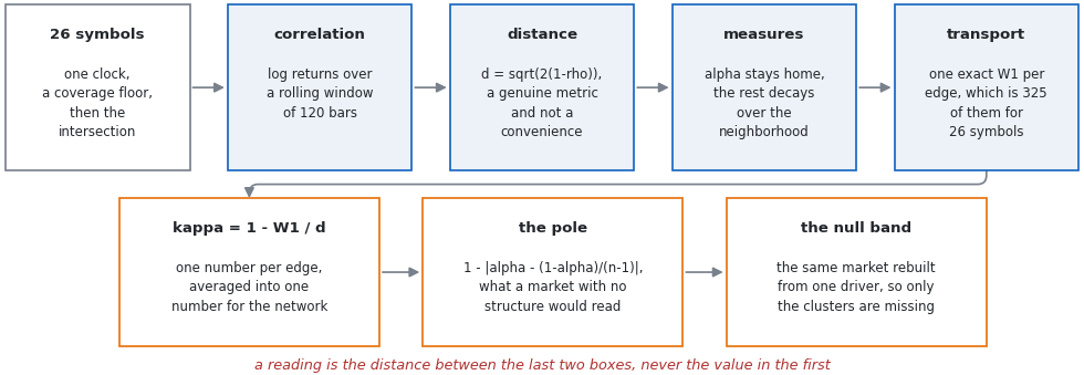
Fig. 1. The six stages, and the fact that a reading is a distance between the last two boxes rather than the value produced by the first

The rest explains how, and what happens when each stage is built the obvious way.

Curvature on a graph, in one formula

Start with the geometry and leave the market out of it. Take a graph, pick an edge between nodes x and y, and give each endpoint a probability measure describing its neighborhood: a share alpha of the mass stays on the node, and the remaining 1 - alpha is spread over its neighbors. Now ask how expensive it is to turn m_x into m_y, where moving one unit of mass from u to v costs d(u, v). That cost is the Wasserstein-1 distance, and Ollivier's curvature compares it to the distance between the nodes.

If the neighborhoods overlap heavily, most of the mass is already where it needs to be, so W1 is much smaller than d and kappa is positive. If the edge is the only route between two otherwise separate groups, every unit has to cross it and then travel further, so W1 exceeds d and kappa goes negative. The measure is what makes this work, and the library builds it from the definition.

//+------------------------------------------------------------------+
//| One probability measure per node, over its own neighborhood      |
//|                                                                  |
//|     m_x(x) = alpha                                               |
//|     m_x(y) = (1 - alpha) w(x,y) / sum_z w(x,z)                   |
//|                                                                  |
//|  A node with no neighbors keeps all of its mass, which makes the |
//|  transport against it well defined instead of a divide by zero.  |
//+------------------------------------------------------------------+
void CORCCurvature::BuildMeasures(const double &dist[], const bool &adj[],
                                  const double h)
  {
   int    n  = m_n;
   double h2 = 2.0 * h * h;
   if(h2 <= ORC_CEPS)
      h2 = 2.0;
 
   for(int x = 0; x < n; x++)
     {
      int base = x * n;
      for(int i = 0; i < n; i++)
         m_meas[base + i] = 0.0;
 
      double total = 0.0;
      for(int y = 0; y < n; y++)
        {
         if(y == x || !adj[base + y])
            continue;
         double w = 1.0;
         if(m_weighting == ORC_W_DECAY)
           {
            double d = dist[base + y];
            w = MathExp(-d * d / h2);
           }
         m_meas[base + y] = w;
         total += w;
        }
 
      if(total <= ORC_CEPS)
        {
         m_meas[base + x] = 1.0;         // isolated node keeps its mass
         continue;
        }
 
      double share = (1.0 - m_alpha) / total;
      for(int y = 0; y < n; y++)
         if(m_meas[base + y] > 0.0)
            m_meas[base + y] *= share;
      m_meas[base + x] = m_alpha;
     }
  }

The isolated node case is not defensive clutter. A node with no neighbors keeps all of its mass, which makes the transport against it well defined instead of a division by zero, and the sparse graph modes can produce exactly that situation.

Four small graphs pin the sign convention down, and all four have answers that can be worked out by hand, which makes them a test.

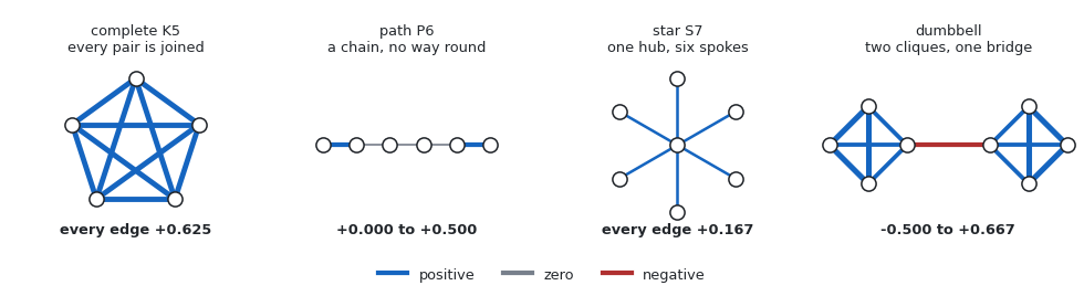
Fig. 2. Edge curvature on four shapes at alpha 0.5, drawn from the same routine the tests use: red is negative, grey is zero, blue is positive

On the complete graph every edge reads exactly +0.625, because every pair of neighborhoods is identical. Along a path the interior edges read 0.000 and the end edges +0.500. Every spoke of the seven-node star reads +0.166667. The dumbbell is the finance argument in miniature: two cliques joined by one bridge, where the bridge reads -0.500000 and the clique edges average +0.541667. That bridge is the only way across, so its removal splits the market, and the curvature says so with a sign change rather than a threshold.

Translating this to markets needs a distance, and the standard one comes from Mantegna's 1999 work on correlation-based trees: d(i, j) = sqrt(2 (1 - rho)). Perfectly correlated instruments sit at distance 0, uncorrelated ones at sqrt(2), and perfectly anticorrelated ones at 2. This transform is not a convenience: it is a genuine metric, and two parts of the library are correct only because it satisfies the triangle inequality. The class exposes WorstTriangleSlack() and the tests assert on it, so swapping in another distance formula has to clear that assertion or two speedups silently stop being exact.

The transport problem, solved exactly

W1 between two discrete measures is a transportation problem, a minimum cost flow, and the textbook method is successive shortest augmenting paths with node potentials. There is no iteration count to tune, no convergence tolerance to pick and no regularization weight: the answer that comes back is the answer, and the solver can prove it. There are small fixed epsilons, ORC_EPS, ORC_CEPS and ORC_GEPS at 1.0e-12 and a 1.0e-10 floor on flow read back, but they decide when a residual counts as spent rather than how accurate the answer is, and the certificate does not depend on them. The entropic approximation trades exactness for speed on problems with tens of thousands of points; these have 26.

One property is where the speed comes from. Wherever the two measures already agree, that mass can stay where it is, so only the difference has to be transported:

W1(a, b) = W1( (a-b)+ , (b-a)+ )

//+------------------------------------------------------------------+
//| Wasserstein-1 between two measures over the same node set        |
//|                                                                  |
//|  mx and my are full length probability vectors over n nodes and  |
//|  cost is the n x n metric between those nodes. Only the parts    |
//|  where the two disagree are handed to the solver; see the class  |
//|  header for why that is exact and what it buys.                  |
//+------------------------------------------------------------------+
double CORCTransport::Wasserstein(const double &mx[], const double &my[],
                                  const double &cost[], const int n)
  {
   if(ArraySize(m_supply) < n)
     {
      ArrayResize(m_supply, n);
      ArrayResize(m_demand, n);
      ArrayResize(m_supIdx, n);
      ArrayResize(m_demIdx, n);
     }
 
   int m = 0, k = 0;
   for(int i = 0; i < n; i++)
     {
      double d = mx[i] - my[i];
      if(d > ORC_EPS)
        {
         m_supply[m] = d;
         m_supIdx[m] = i;
         m++;
        }
      else
         if(d < -ORC_EPS)
           {
            m_demand[k] = -d;
            m_demIdx[k] = i;
            k++;
           }
     }
 
   if(m == 0 || k == 0)
     {
      m_solved     = true;
      m_ownProblem = false;
      m_m = 0;
      m_n = 0;
      return(0.0);                        // the measures already agree
     }
 
   int need = m * k;
   if(ArraySize(m_block) < need)
      ArrayResize(m_block, need);
   for(int i = 0; i < m; i++)
      for(int j = 0; j < k; j++)
         m_block[i * k + j] = cost[m_supIdx[i] * n + m_demIdx[j]];
 
   double w1 = SolveDense(m_supply, m_demand, m_block, m, k);
   m_ownProblem = (w1 >= 0.0);
   return(w1);
  }

Measured on the library's own test data, that reduction takes a typical instance from 99 linear program variables to 24, a shrink of 4.17 times, and cuts the mass that has to move from 1.0 to a median of 0.47 at the shipped alpha of 0.5. It is exact only when the cost is a metric, which is why the Mantegna transform earns its place. The test suite measures that dependency: on the Mantegna distance the full and reduced answers agree to 0.000e+00, and on a cost matrix built to violate the triangle inequality the same shortcut is wrong by up to 2.039e-01.

The solver loop is short, and the line that matters most in it is the iteration guard.

   //--- successive shortest augmenting paths
   double total = 0.0;
   double distT = 0.0;
   // The classical m+n bound does NOT hold: an arc carrying flow has
   // reduced cost zero, so a shortest path may walk its reverse and
   // saturate that instead. Measured over 62 400 solves the mean is
   // 1.5(m+n) and the tail runs past 2(m+n). The limit below is an
   // empirical backstop against a cycle, not a proved bound, which is
   // why HitGuard() is reported rather than silently absorbed.
   int    guard = 16 * (m + n) + 64;
 
   while(m_augmentations < guard)
     {
      if(!Dijkstra(src, snk, distT))
         break;
 
      for(int i = 0; i < m_nodes; i++)
         m_pot[i] += (m_dist[i] < DBL_MAX ? m_dist[i] : distT);
 
      //--- bottleneck along the path
      double push = DBL_MAX;
      int    v    = snk;
      while(v != src)
        {
         int e = m_prevArc[v];
         if(e == ORC_ARC_NONE)
            return(-1.0);
         if(m_cap[e] < push)
            push = m_cap[e];
         v = m_to[e ^ 1];
        }
      if(push < m_smallestPush)
         m_smallestPush = push;
      if(push <= ORC_EPS)
         break;
 
      //--- apply it, accumulating the TRUE cost, not the reduced one
      v = snk;
      while(v != src)
        {
         int e = m_prevArc[v];
         m_cap[e]     -= push;
         m_cap[e ^ 1] += push;
         total        += m_cost[e] * push;
         v = m_to[e ^ 1];
        }
      m_augmentations++;
     }
 
   // Hitting the guard means the loop stopped counting, not that the
   // flow is complete, so the number in hand is not a solution. It is
   // refused rather than returned: a wrong W1 becomes a wrong kappa,
   // and a wrong kappa is indistinguishable from a market reading.
   m_hitGuard = (m_augmentations >= guard);
   if(m_hitGuard)
      return(-1.0);
 
   m_solved = true;
   return(total);
  }

The classical bound for a transportation problem is m + n augmentations, one for each supply or demand that gets saturated. That bound does not hold here: by complementary slackness every arc carrying flow has reduced cost exactly zero, so its reverse arc is free to walk, and a shortest path can saturate one of those instead of a supply or a demand. How far past the bound it goes is a measurement, and ORC_Probe_Solver.mq5 is what takes it.

[ORC] ==== solver probe start, n=30 ====
[ORC] n=12  solved  2640  REFUSED    0  bad certs 0  worst cert 1.554e-15  aug mean 13.6 max 24  minpush 2.7e-08
[ORC] n=18  solved  6120  REFUSED    0  bad certs 0  worst cert 1.721e-15  aug mean 23.2 max 42  minpush 2.2e-09
[ORC] n=24  solved 11040  REFUSED    0  bad certs 0  worst cert 2.220e-15  aug mean 33.3 max 67  minpush 7.9e-10
[ORC] n=30  solved 17400  REFUSED    0  bad certs 0  worst cert 2.831e-15  aug mean 44.0 max 88  minpush 3.0e-10
[ORC] n=36  solved 25200  REFUSED    0  bad certs 0  worst cert 3.109e-15  aug mean 55.2 max 116  minpush 3.0e-11
[ORC] OVERALL solved 62400, REFUSED 0 (0.00%), bad certificates 0, worst certificate 3.109e-15
[ORC] ==== solver probe done ====

Read the augmentation columns relative to the problem size. The reduced transport problem for an n-symbol network has about n supplies and demands between them, so the mean sits at roughly 1.5 times (m + n) and the maximum at 3.2 times at the largest size, and the ratio is still creeping upward as the network grows. The classical bound is passed on essentially every solve, and no fixed multiple of it is safe to assume.

That is what sets the guard. A limit of 2(m + n) sits below the observed maximum, and reaching a limit does not complete the flow, it only stops the loop counting: recompiled with that limit, the same sweep leaves 5 edges at n = 24, 70 at n = 30 and 424 at n = 36 failing the certificate, the worst by 4.891e-01. A residual that size is the whole signal this library measures, so such a solve is arithmetic wearing the format of a result. The shipped guard is 16(m + n) + 64, set from the sweep with room to spare: an empirical backstop against cycles, not a proved bound. If it is hit, the solver refuses and returns -1.0, because an inexact kappa is indistinguishable from a market reading.

None of that would be measurable without the unusual part: the solver certifies itself.

//+------------------------------------------------------------------+
//| An optimality certificate the solver produces about itself       |
//|                                                                  |
//|  Returns the largest violation of the three conditions that,     |
//|  together, mean the answer is optimal and not merely feasible:   |
//|                                                                  |
//|    1. the plan is feasible - every row sums to its supply and    |
//|       every column to its demand;                                |
//|    2. dual feasibility - pot[j] - pot[i] <= c(i,j) everywhere;   |
//|    3. complementary slackness - wherever mass actually moved,    |
//|       that inequality is tight.                                  |
//|                                                                  |
//|  The certificate needs no second implementation to be right, so a|
//|  test can demand a residual near zero on data no reference solver|
//|  covers. It does not replace an external check: it runs on the   |
//|  same code path and the same data, so it can only catch a plan   |
//|  this solver got wrong, never a shared misreading of the problem.|
//|  That is what the HiGHS crosscheck is for.                       |
//+------------------------------------------------------------------+
double CORCTransport::Certify(const double &supply[], const double &demand[],
                              const double &cost[], const int m,
                              const int n) const
  {
   if(!m_solved)
      return(DBL_MAX);
 
   double worst = 0.0;
 
   for(int i = 0; i < m; i++)
     {
      double row = 0.0;
      for(int j = 0; j < n; j++)
         row += Flow(i, j);
      worst = MathMax(worst, MathAbs(row - supply[i]));
     }
   for(int j = 0; j < n; j++)
     {
      double col = 0.0;
      for(int i = 0; i < m; i++)
         col += Flow(i, j);
      worst = MathMax(worst, MathAbs(col - demand[j]));
     }
 
   for(int i = 0; i < m; i++)
      for(int j = 0; j < n; j++)
        {
         double slack = cost[i * n + j] - (m_pot[m + j] - m_pot[i]);
         if(slack < 0.0)
            worst = MathMax(worst, -slack);              // dual infeasible
         if(Flow(i, j) > 1.0e-10)
            worst = MathMax(worst, MathAbs(slack));      // must be tight
        }
 
   return(worst);
  }

Three conditions together mean the answer is optimal, not merely feasible: the plan moves exactly the supplies and fills exactly the demands, the dual inequality holds everywhere, and it is tight wherever mass moved. The value is that it needs no reference implementation: there is no external oracle for 62 400 random transport instances, so a test can demand a near zero residual on data no reference covers. At the shipped guard the worst residual across that sweep is 3.109e-15, with zero refusals and zero bad certificates. It does not replace an external check. Running on the same code path and arrays as the solve, it catches a plan this solver got wrong but never a misreading both share, which is why the HiGHS crosscheck exists and why the sweep is evidence about the instances tested, not a proof for every input.

Twenty-six symbols on one clock

Most indicators read one symbol. This one reads twenty-six, and that is a different problem. A correlation is only meaningful between returns observed over the same interval, so the usable sample is the intersection of the symbols' bar times, not the union and not the longest member. Two consequences were measured on a live broker.

First, the basket's start date is set by its worst member. On daily bars, FX and metals reached back nine years, crypto seven, indices six, and one energy symbol only five, so adding that symbol would have cost every other one four years of history. Second, a symbol on a slightly different calendar deletes rows for the whole basket: across 47 candidates only 1347 of 1702 bar times were common, so 21% of the sample was gone, almost all of it from four symbols, the worst at 86.0% coverage.

Coverage is therefore computed per symbol, offenders are dropped before the intersection, and the reason is kept. The subtlety is what coverage is measured against.

   //--- pass one: coverage measured ONLY over the calendar the two
   //--- histories share, so a different trading calendar, which
   //--- deletes rows for everybody, is not confused with a later
   //--- start, which the intersection already handles. Measured the
   //--- other way, crypto left the basket at 85.5% for being younger.
   int anchor = AnchorOf(false);
   if(anchor < 0)
      return(false);
 
   int      an     = m_series[anchor].count;
   datetime aFirst = m_series[anchor].t[0];
   datetime aLast  = m_series[anchor].t[an - 1];
 
   for(int i = 0; i < m_requested; i++)
     {
      if(m_series[i].count <= 0)
         continue;
 
      datetime lo = MathMax(aFirst, m_series[i].t[0]);
      datetime hi = MathMin(aLast, m_series[i].t[m_series[i].count - 1]);
 
      int inRange = 0, hit = 0;
      for(int b = 0; b < an; b++)
        {
         datetime t = m_series[anchor].t[b];
         if(t < lo || t > hi)
            continue;
         inRange++;
         if(HasTime(m_series[i].t, m_series[i].count, t))
            hit++;
        }
 
      m_series[i].coverage = (inRange > 0 ? (double)hit / inRange : 0.0);
      m_series[i].used     = (m_series[i].coverage >= m_minCoverage &&
                              inRange >= 2);
      if(!m_series[i].used)
         m_series[i].reason = StringFormat("coverage %.1f%% of the %d shared "
                                           "bar times, below the %.1f%% floor",
                                           100.0 * m_series[i].coverage,
                                           inRange, 100.0 * m_minCoverage);
     }

Measuring coverage over the anchor's whole range would conflate two different faults. A symbol on a different calendar deletes rows from everyone and has to go. A symbol that simply starts later only costs the basket a start date, which the intersection already handles. Asking a broker for a fixed 1200 daily bars gives a seven day a week instrument about 3.3 years and a five day a week one about 4.2, so measured that way crypto scores 85.5% and leaves for being younger rather than misaligned. Restricting the comparison to the calendar span the two histories share keeps it.

The 97% floor that ships is a daily setting; below D1 it deletes the entire point of the basket. On thirty minute bars every metal, every index and oil score 94% to 95% against FX, because their sessions differ, so a 0.97 floor drops 11 of 26 symbols and leaves an FX only network wearing a multi-asset label. On M30 over 2000 bars: 0.97 gives 15 symbols and 1423 rows, while 0.90 gives all 26 for 1322 rows, so the whole multi-asset structure costs 7% of the rows. Use 0.90 intraday, and the class appends a warning to its note whenever a fifth or more of the basket is lost, because a panel row saying "15 of 26" is easy to read straight past.

Important: a partial basket is not a smaller basket, it is a different network. Fewer nodes move the structureless pole, change every measure and change the answer, so accepting whichever symbols happen to have arrived would report a curvature for twenty-six names while reading sixteen. The class separates "still downloading" from "genuinely dropped" through PendingCount(), and the indicator refuses to compute until that count is zero.

There is a platform constraint underneath that, worth naming for anyone writing multi-symbol code. Sleep does not work in a custom indicator, so a retry loop around CopyRates with a sleep between attempts spins instantly, finds nothing, and reports that the broker offers no history when the series is merely still arriving. The class reads MQL_PROGRAM_TYPE and asks once in an indicator, marking the miss as pending so the caller can retry later.

The two decisions that decide whether the number means anything

Two choices sit between the definition and a usable gauge, and in each case the obvious option carries no information. Neither is settled by taste: each has a closed form or a measurement.

The graph, and a closed form that kills the obvious design. The natural first move is to make every pair an edge and give every neighbor an equal share of the mass. On a complete graph with a uniform measure, m_x and m_y agree on every node except x and y, so exactly |alpha - (1-alpha)/(n-1)| of mass has to move, and it moves exactly d(x, y). The distance cancels:

//+------------------------------------------------------------------+
//| What a market with no structure at all would read                |
//|                                                                  |
//|  A complete graph with a flat measure gives exactly this value,  |
//|  and it depends only on the node count and on alpha. It is the   |
//|  POLE of the scale: real readings sit just below it, and the gap |
//|  rather than the level is what carries information. A line drawn |
//|  at 0.47 says nothing; the same reading as a gap of 0.046 does.  |
//+------------------------------------------------------------------+
double CORCGraph::StructurelessReference(const int n, const double alpha)
  {
   if(n < 2)
      return(1.0);
   return(1.0 - MathAbs(alpha - (1.0 - alpha) / (double)(n - 1)));
  }

That configuration cannot see the market at all. It is not a tendency but an identity: confirmed at 5, 8 and 12 nodes and at alpha 0, 0.25, 0.5 and 0.75, the worst error against the closed form is 9.992e-16 and the spread across edges is 2.220e-16. What the gauge needs is therefore not sparsity but a measure that is not uniform: a near neighbor must carry more mass than a far one, or the distances cancel and the reading is a constant.

The obvious repair, making the graph sparse, is worse. Two genuine sectors make a k-nearest-neighbor graph or a threshold graph fall into separate components, so shortest paths become infinite and W1 is undefined on exactly the market this method exists to detect. The k-nearest variant has a second flaw: it only reacts once the neighbor ordering changes, which makes it a step detector, flat from an inter-sector correlation of 0.0 to 0.6 and then jumping.

The shipped design gives the two roles to two different objects. The cost stays the full Mantegna metric, so it is always finite, and no shortest path pass is needed because on a complete graph over a metric the direct arc is already cheapest. The measure is what becomes non uniform, giving a closer neighbor more mass through a Gaussian decay.

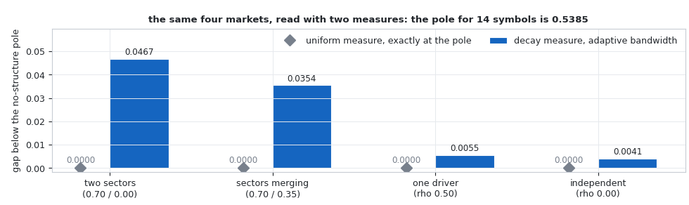
Fig. 3. The same four markets under both measures: the uniform measure returns the pole exactly, whatever the market, while the decay measure separates two sectors from one driver by an order of magnitude

The bandwidth, and how a fixed one smuggles the level back in. A Gaussian decay needs a width, and the tempting choice is a constant. A fixed width is fixed in distance units, so when every correlation rises every distance shrinks, every weight approaches one, and the measure flattens toward uniform. That drifts the gauge toward the degenerate constant above, which reads as a fragility signal and is really a level signal. Taking the width from the window's own median distance removes the dependence.

//+------------------------------------------------------------------+
//| Mantegna distance, plus the window's own scale                   |
//|                                                                  |
//|  The median off diagonal distance is what makes the decay measure|
//|  scale free. A fixed width in distance units reintroduces the    |
//|  correlation LEVEL through the back door: when everything becomes|
//|  more correlated every distance shrinks, every weight approaches |
//|  one, and the measure flattens toward uniform, which is the      |
//|  degenerate case the whole design exists to avoid. Measured, a   |
//|  fixed width of 0.7 moves kappa by 0.3061 under a doubling of    |
//|  every distance; the median width moves it by 4.4e-16.           |
//+------------------------------------------------------------------+
void CORCGraph::DeriveDistance(void)
  {
   int n = m_n;
   for(int i = 0; i < n; i++)
     {
      m_dist[i * n + i] = 0.0;
      for(int j = i + 1; j < n; j++)
        {
         double arg = 2.0 * (1.0 - m_corr[i * n + j]);
         if(arg < 0.0)
            arg = 0.0;
         double d = MathSqrt(arg);
         m_dist[i * n + j] = d;
         m_dist[j * n + i] = d;
        }
     }
 
   int    cnt = 0;
   double sum = 0.0;
   double off[];
   ArrayResize(off, n * (n - 1) / 2);
   for(int i = 0; i < n; i++)
      for(int j = i + 1; j < n; j++)
        {
         off[cnt++] = m_dist[i * n + j];
         sum += MathAbs(m_corr[i * n + j]);
        }
   ArraySort(off);
   m_bandwidth = (cnt > 0 ? off[cnt / 2] : 1.0);
   if(m_bandwidth <= ORC_GEPS)
      m_bandwidth = 1.0;
   m_meanAbsCorr = (cnt > 0 ? sum / cnt : 0.0);
  }

Measured under a doubling of every distance in the matrix, a fixed bandwidth of 0.7 moves kappa by 0.3061, while the window's own median moves it by 4.4e-16. That is not a smoothing preference, it is the difference between a scale-free statistic and one that tracks the correlation level.

Three curvature aggregates appear below and only one is the reading. Kappa is the unweighted mean over every scored edge, all 325 on a twenty-six symbol basket, and it is what the gap is measured from and what the nulls are compared against. Node curvature is the mean over a symbol's own edges, the only form an expert can act on instrument by instrument. The struct also carries kappaWeighted, each edge weighted by its absolute correlation, and nothing consumes it: it is a diagnostic, since weighting by correlation would reintroduce the level dependence the two decisions remove.

With both decisions made correctly the central claim can be tested, narrowly. Curvature is a ratio of a distance to a distance and W1 is linear in the cost matrix, so multiplying every distance by one constant leaves kappa bit-identical. That is a proof about rescaling, and rescaling is not what a rising market does: Mantegna's map is concave, so adding 0.05 to every correlation shortens an edge at rho 0.9 by 29% and one at rho 0.1 by 2.8%. The network is bent, tight part compressed hardest, not scaled. What survives is a measurement, not a corollary.

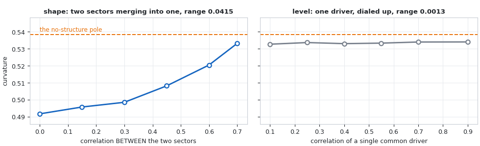
Fig. 4. Two sectors merging move the gauge by 0.0415 across six points, while a single driver dialed from rho 0.1 to 0.9 moves it by 0.0013, which is sampling noise between independent draws rather than a response

The library's own test runs a tighter version of the same pair, three points each with matched seeds, measuring the shape sweep at 0.0415 against a level sweep 261 times smaller, printed as 0.0002. At a fixed shape, dialing the level moves the gauge by about what resampling noise moves it, so "everything became more correlated" is close to invisible to this statistic. That is a measured near-invariance on synthetic markets, not a structural one, and the real basket below puts a number on what survives.

The nulls, including the one that is empty

Choosing the null is where most of the thinking went, and the first candidate is instructive because it is completely empty. In the anomaly detection and dependence libraries I have built for this site, the sharpest control is to shuffle the bars in time, destroying only the ordering. That control cannot work here. Permuting the rows of a return matrix leaves every column pair correlation algebraically unchanged, so it produces the identical correlation matrix, distance matrix and curvature: reporting it as a passed control would be reporting that a number equals itself. The data test asserts exactly this, so a control that cannot move the number is never counted as a success: a joint shuffle moves kappa by 0.0e+00, while shuffling each symbol separately moves it by 2.5e-02.

Two nulls do carry information. The independent null permutes each symbol's returns on its own, so every symbol keeps its own distribution, fat tails included, and only the cross-sectional structure is destroyed. At a finite window this does not read as the structureless pole, because sampling noise alone builds correlation, which makes it the honest "no relationships, this many observations" reference. The one-factor null matters more.

//+------------------------------------------------------------------+
//| Null 2: one common driver, no clusters                           |
//|                                                                  |
//|  Calibrated to the window's own average absolute correlation and |
//|  to each symbol's own volatility, and Gaussian in everything it  |
//|  does not match, so it is a no-sector-structure reference rather |
//|  than a market that differs in one respect. That is the          |
//|  comparison the whole method claims to be able to make.          |
//+------------------------------------------------------------------+
bool CORCFragility::NullOneFactor(CORCData &data, const int endRow,
                                  const int window, const int draws,
                                  SORCNullBand &band)
  {
   ZeroMemory(band);
   double ret[];
   if(!data.ReturnsWindow(endRow, window, ret))
      return(false);
 
   int n = data.Symbols();
   if(!m_graph.BuildFromReturns(ret, window, n))
      return(false);
   double rho = m_graph.MeanAbsCorr();
   if(rho < 0.0)
      rho = 0.0;
   if(rho > 0.95)
      rho = 0.95;
 
   //--- each symbol's own volatility, so only the SHAPE differs
   double sd[];
   ArrayResize(sd, n);
   for(int i = 0; i < n; i++)
     {
      double mean = 0.0;
      for(int t = 0; t < window; t++)
         mean += ret[t * n + i];
      mean /= window;
      double s2 = 0.0;
      for(int t = 0; t < window; t++)
        {
         double dv = ret[t * n + i] - mean;
         s2 += dv * dv;
        }
      sd[i] = MathSqrt(s2 / MathMax(window - 1, 1));
     }
 
   double a = MathSqrt(rho);
   double b = MathSqrt(1.0 - rho);
 
   double synth[];
   ArrayResize(synth, window * n);
   double vals[];
   ArrayResize(vals, draws);
   int got = 0;
 
   for(int d = 0; d < draws; d++)
     {
      for(int t = 0; t < window; t++)
        {
         double f = m_rng.NextNormal();
         for(int i = 0; i < n; i++)
            synth[t * n + i] = sd[i] * (a * f + b * m_rng.NextNormal());
        }
 
      SORCNetwork net;
      if(CurvatureOf(synth, window, n, net))
         vals[got++] = net.kappaMean;
     }
 
   Summarize(vals, got, band);
   return(band.valid);
  }

It regenerates the window from a single common driver calibrated to the window's own average absolute correlation, giving each synthetic symbol that symbol's own volatility. The result is a market that is correlated, sometimes heavily, with no cluster structure. Because curvature moves very little with the level, a market that has merely become more correlated should land near this band, and one that has genuinely lost its sector structure should leave it. That is the comparison the method claims to make, and the only one the display is built around.

[ORC] == 3. the nulls ==================================
[ORC] a joint time shuffle is NOT used: permuting rows of a return matrix leaves every correlation unchanged.
[ORC] date              real     indep  1-factor   z vs 1f  avg|rho|
[ORC] 2020.01.14    0.475956  0.508619  0.508541     -73.8     0.304
[ORC] 2021.09.22    0.475726  0.508588  0.508392     -70.3     0.383
[ORC] 2023.06.05    0.477699  0.508401  0.508431     -49.1     0.300
[ORC] 2025.01.08    0.478893  0.508419  0.508606     -63.2     0.302
[ORC] 2026.08.13    0.465475  0.508447  0.508266     -83.0     0.415
[ORC] mean z against the one factor null: -67.9 sd
[ORC] windows below BOTH nulls' 5th percentile: 5 of 5
[ORC] reading: a real market sitting far below the one factor band still has sector structure; a market drifting up into the band has lost it.

Five points across six and a half years, twenty draws each. Real curvature sits 49 to 83 standard deviations below the one-factor band, and 5 of 5 windows fall below the fifth percentile of both nulls. Read the sd figures as an order of magnitude: twenty draws fix the band's mean well and its spread only roughly, so what they support is "far outside the null" rather than "-67.9" as a measured quantity, while the 5 of 5 count needs no spread estimate. The null is a reference, not a model. Its draw is Gaussian on one positive factor, so it reproduces neither the real tails nor the negative pairs a real basket carries, and another matrix with the same average absolute correlation could have a different spectrum. What survives is the direction: a real matrix is not a blob.

One more thing travels with every reading. A high curvature is ambiguous, because a market with almost no relationships and one collapsed into a single undifferentiated blob both lack cluster structure. The level sweep measures it on a fourteen node synthetic basket: at rho 0.1 it reads 0.533545 and at rho 0.9 it reads 0.533490. The scale depends on the basket size: fourteen nodes put the pole at 0.538462 rather than the 0.520000 of the twenty-six symbol basket, so both sit about 0.005 below their own pole, not above it. Only the average correlation separates the two cases, which is why the band is a floor to stay below rather than a target, and why every reading carries meanAbsCorr.

What real markets read

Start with a single window, because it shows what the aggregate is averaging over: the most recent 120 bar window of the twenty-six symbol basket, taken from the file the export script writes and re-solved in Python.

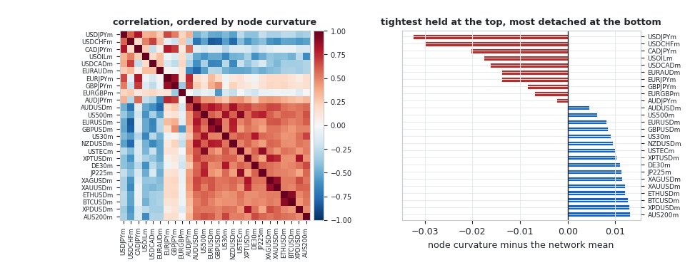
Fig. 5. The correlation matrix of one window with symbols ordered by node curvature, and the same ordering as a bar chart: the block structure the gauge responds to is the red square lower right and the group opposing it upper left

The ordering is the interesting part. The most tightly held members are USDJPY at 0.4330 and USDCHF at 0.4354, roughly 0.032 below the network mean, followed by CADJPY, oil and USDCAD; the most detached are AUS200, palladium, Bitcoin and Ethereum, about 0.013 above it. That is a node level reading, the only form an expert could act on symbol by symbol. Nothing about it is a forecast: it says which instruments sit inside the tight part of the network.

Rolling it through history gives the picture the indicator plots.

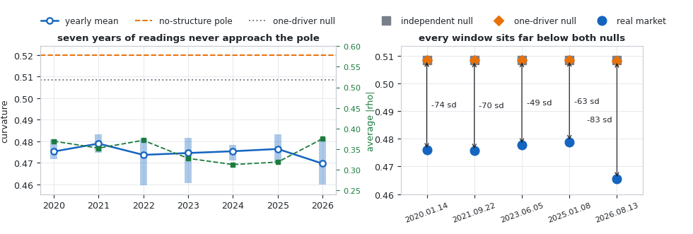
Fig. 6. Left, the yearly range of readings with the average correlation on the second axis; right, the five null points, each real window sitting between 49 and 83 standard deviations below its one-driver band

The year table underneath lets a named event be looked up rather than inferred from extremes.

Year	Windows	kappa min	kappa mean	kappa max	avg |rho|
2020	55	0.471721	0.475219	0.480969	0.369
2021	57	0.474633	0.478921	0.483299	0.352
2022	57	0.459595	0.473677	0.481340	0.371
2023	58	0.460508	0.474541	0.481651	0.327
2024	60	0.471216	0.475362	0.478367	0.312
2025	60	0.470394	0.476422	0.483143	0.318
2026	38	0.459848	0.469638	0.481259	0.375

March 2020 does not produce the extreme reading, and that is a result rather than an omission. The 2020 row reads a mean of 0.4752 against a full sample mean of 0.4751, which is mid-pack. The most clustered windows are December 2022, January 2023 and mid 2026; the least clustered are April and May 2021, and February and March 2025. The largest systemic shock in the sample is close to invisible here. That is consistent with a crisis raising correlations without dissolving the sector map, but it is a reading rather than a demonstrated cause: a 120 bar daily window spans six months, averaging the crash with the recovery. Both explanations predict a mid-pack row and this table cannot separate them.

Two further measurements complete the description. The first answers the objection that this is a relabelling of average correlation: over the 385 rolling windows the Pearson correlation between the two is -0.746 and the Spearman is -0.697. They are strongly related, and the variance left over around that straight line is 44.4%. Read that narrowly: it is what a linear fit on the average correlation fails to reproduce, not a measured independent signal, and a nonlinear function of the average could claim some of it. Each window also shares 115 of its 120 bars with the next, so the effective sample behind -0.746 is well under 385. The scan prints a warning if the rank agreement ever exceeds 0.95, because past that point the two are the same statistic on this basket.

The second asks what follows a reading. Splitting all 381 usable windows at their own median and measuring the next 20 bars of an equally weighted basket: the more clustered half is followed by a forward realized volatility of 0.006091 and a drawdown of 0.022798, the less clustered half by 0.006573 and 0.029660. The ratio is 1.079, and it points the opposite way from the obvious story, since slightly less cluster structure precedes slightly more volatility. Consecutive windows share bars, so an effect of 8% on overlapping samples is not something to build on. It is reported because it is what the data says.

The indicator, and the expert

Everything above sits behind one class, so a caller never touches a transport solver.

class CORC
  {
private:
   CORCData          m_data;
   CORCFragility     m_frag;
   int               m_window;
   bool              m_loaded;
 
public:
                     CORC(void);
 
   //--- setup
   bool              Load(const string symbolsCsv, const ENUM_TIMEFRAMES tf,
                          const int bars);
   void              SetMinCoverage(const double v) { m_data.SetMinCoverage(v); }
   void              SetAlpha(const double a)       { m_frag.SetAlpha(a);       }
   void              SetWeighting(const ENUM_ORC_WEIGHTING w)
     {
      m_frag.SetWeighting(w);
     }
   void              SetSeed(const ulong s)         { m_frag.SetSeed(s);        }
 
   //--- readings
   bool              ReadAt(const int endRow, const int window,
                            SORCReading &out);
   bool              ReadLatest(const int window, SORCReading &out);
   bool              Scan(const int window, const int step,
                          const int firstRow, const int lastRow);
 
   //--- nulls
   bool              NullIndependent(const int endRow, const int window,
                                     const int draws, SORCNullBand &band);
   bool              NullOneFactor(const int endRow, const int window,
                                   const int draws, SORCNullBand &band);
   static double     StandardScore(const SORCNullBand &band, const double v)
     {
      return(CORCFragility::StandardScoreOf(band, v));
     }
 
   //--- what a caller needs in order to distrust the answer
   double            Pole(void) const;
   string            Verdict(const SORCReading &r, const SORCNullBand &oneFactor)
   const;
 
   //--- pass through
   int               Symbols(void)   const { return(m_data.Symbols());   }
   int               Rows(void)      const { return(m_data.Rows());      }
   int               Requested(void) const { return(m_data.Requested()); }
   bool              Ready(void)     const { return(m_loaded);           }
   string            Note(void)      const { return(m_data.Note());      }
   string            SymbolList(void) const { return(m_data.SymbolList()); }
   string            DroppedReport(void) const { return(m_data.DroppedReport()); }
   int               DroppedCount(void) const { return(m_data.DroppedCount()); }
   int               PendingCount(void) const { return(m_data.PendingCount()); }
   string            Name(const int c) const { return(m_data.Name(c));    }
   double            Coverage(const int c) const { return(m_data.Coverage(c)); }
   datetime          Time(const int r) const { return(m_data.Time(r));    }
   int               ScanCount(void) const { return(m_frag.Count());      }
   int               Refused(void)   const { return(m_frag.Refused());    }
   bool              ScanAt(const int i, SORCReading &out) const
     {
      return(m_frag.At(i, out));
     }
   CORCData         *Data(void) { return(GetPointer(m_data)); }
  };

Load a basket, ask for a reading, ask for a null, and read the gap. Symbols() and DroppedReport() are there so a caller finds out that the basket is not what was asked for rather than wondering why the scan is short.

ORC_Fragility.mq5 plots the curvature in a subwindow with the one-factor band as two dotted levels, and a panel carrying the average correlation, the gap from the pole, the standardized distance from the band and a verdict. Three properties of that display were each a decision.

1. The plot is a step. One window over twenty-six symbols is 325 exact transport problems, so the reading is computed every InpStep bars and held in between. A held bar carries the previous reading, not an interpolation, and the reading changes on average every 5.3 bars against a declared step of five.
2. The band is computed once, at the newest bar, and drawn as levels. A null draw costs a full curvature computation, so fifteen draws cost fifteen windows: affordable once, not per bar.
3. Every plotted point comes from its own causal window and is never revisited. The indicator walks chart bars and assigns the newest reading at or before each one, because the basket is an intersection with fewer rows than the chart has bars. Stepping over basket rows instead leaves a hole at every bar the basket does not contain.

Important: the first load is expensive and it is meant to be. On a twenty-six symbol basket, 81 computed windows across 201 plotted bars took 15.2 seconds on a cold start and 6.9 to 9.8 seconds once the histories were cached. Raising InpHistoryBars is the fastest way to make the chart look frozen. A single window costs 83 ms at 26 symbols, 23 ms at 20 and 4.2 ms at 14 on an idle terminal, so the basket size dominates and is roughly cubic. The scan in section 2 reports 137 ms for the same window off the same meter, because it ran with charts working beside it.

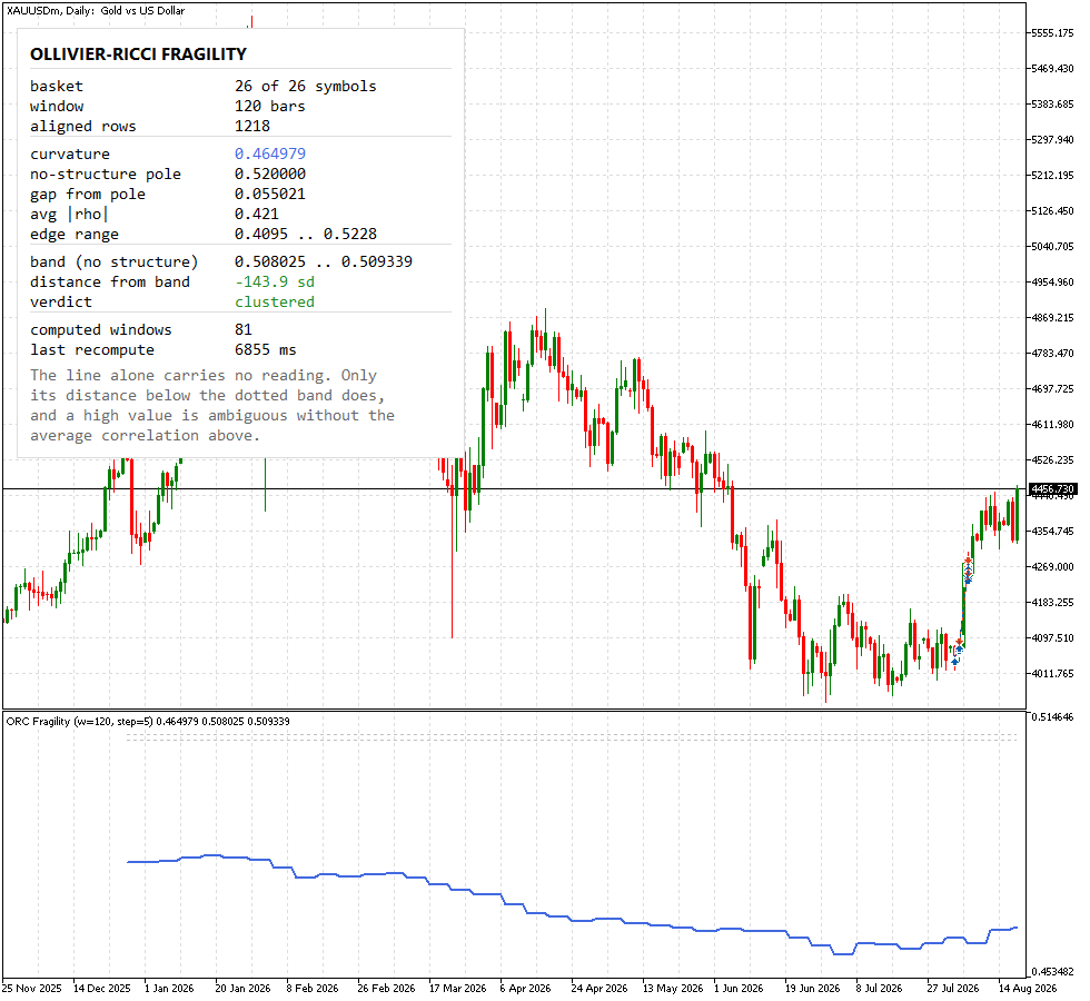
Fig. 7. The indicator on XAUUSDm daily bars with the full 26 symbol basket: the blue step is the curvature, the dotted pair is what the same market would read with no cluster structure, and the reading is the distance between them, here 0.055 below the pole and 143.9 standard deviations below the band

ORC_RiskOff_EA.mq5 is a demonstration and no profit is claimed for it. Curvature describes the geometry of a whole market, so it says nothing about the next bar of any one instrument and cannot be an entry signal. A plain Donchian breakout supplies the entries; the network reading only decides whether to take them.

Its one non-obvious design point is the gate threshold. The usual habit would be to demand that the reading clear the null band by, say, 1.5 standard deviations. Real readings clear it by 49 to 142 standard deviations, so that test is always true: on a daily run it refuses 0 of 82 signals while looking like a working filter. The distance scale depends on the basket, the window and the number of null draws, and cannot be guessed. The shipped gate is therefore a percentile of the gauge's own recent history, with the null distance kept as a validity floor, and on that same run it refuses 102 of 144 signals.

On XAUUSD thirty minute bars, and on that symbol alone, the gate behaves the way a risk gate should:

Arm	Trades	Net	Profit factor	Per trade	Balance drawdown	Sharpe
Gate off	230	16 761	1.33	72.88	25.21%	3.52
Skip when structure is lost	126	11 134	1.57	88.36	15.78%	4.78
Skip when tightly clustered	108	2 589	1.17	23.97	23.42%	1.86

Lower return, much lower drawdown, better on every risk-adjusted column, and the opposite arm is worse on all of them, which is the control that stops "it simply traded less" from explaining the result. It is also one symbol, and the identical configuration does not repeat it. On daily bars across five symbols the ordering holds cleanly on two, partly on a third, and reverses on the remaining two. On thirty minute bars across four, two hold, one gives the drawdown reduction without the ordering, and one reverses. With that few symbols and three orderings, that is about what chance produces.

The expert is therefore a worked example of how the reading can be consumed, and no edge is claimed for it. That conclusion is available only because the three arm test was run across symbols instead of stopping at the one that looked good. A single symbol backtest is a hypothesis, not a finding.

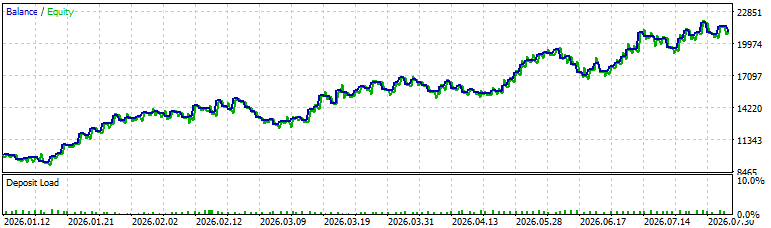
Fig. 8. The gated arm of the demonstration expert, XAUUSDm M30 from January to August 2026 with the full 26 symbol basket at a 480 bar window: 126 trades from 440 signals, the other 314 refused by the gate. A worked example of consuming the reading, not a strategy result

Verification

The reference implementation for this method is GraphRicciCurvature, and it cannot be installed here: it needs POT, POT has no wheel for this Python version, and building it needs a C compiler this machine does not have. The verification is therefore self-contained, and anchored more heavily than it would have been with an oracle.

W1 is checked four independent ways, all reproducing to machine epsilon in both languages.

• Against a closed form with no optimization in it. With the support on a line and cost equal to the absolute difference, W1 is the integral of the absolute difference of the cumulative distributions. Worst error 1.776e-15.
• Against the Kantorovich dual, posed and solved separately. Reading the primal solver's multipliers would prove nothing. Worst duality gap 9.992e-16.
• Against brute force over every permutation. When both measures are uniform over k atoms the optimum sits at a permutation, so trying all k! of them is exact. Worst error 0.000e+00.
• Against the solver's own optimality certificate, on data no reference covers. Worst residual 1.305e-15 in the test suite and 3.109e-15 across the 62 400 solve sweep.

The curvature layer is anchored on the closed-form shapes of Fig. 2: the complete graph identity to 9.992e-16 with an edge spread of 2.220e-16, the path interior at exactly zero, the branching tree inner edge at exactly -2/3, and the star spokes with a spread of 0.000e+00. Scale invariance under the adaptive bandwidth comes out at 4.441e-16, and the same check with a fixed bandwidth is asserted to fail, because the second half is what makes the first worth having.

Level 3 exports the whole pipeline at full precision and rebuilds it in Python, where every edge is re-solved with scipy's HiGHS simplex. That solver shares no reasoning with the successive shortest path method in the library: one walks shortest paths in a residual graph, the other pivots on a simplex tableau. Two implementations of the same algorithm can agree on a shared mistake; these cannot.

  worst Mantegna distance from the correlation         0.000e+00
  worst adaptive bandwidth                             0.000e+00
  worst correlation from the returns                   4.441e-16
  worst every measure is a probability                 2.220e-16
  worst full vs reduced transport                      1.110e-16
  worst gap                                            3.331e-16
  worst kappa, every edge                              9.992e-16
  worst kappaMax                                       0.000e+00
  worst kappaMean                                      3.331e-16
  worst kappaMin                                       0.000e+00
  worst kappaWeighted                                  0.000e+00
  worst meanAbsCorr                                    0.000e+00
  worst measures from the definition                   6.939e-18
  worst standalone W1 vs HiGHS                         2.220e-16
  worst standalone full vs reduced                     1.665e-16
  worst structureless pole                             0.000e+00
  worst triangle inequality slack                      0.000e+00
  worst uniform stream matches MQL5                    0.000e+00
43 PASS, 0 FAIL  [ALL PASS]

The random number generator deserves a note. MathRand is unusable here on two counts: it returns 15 bits and its state cannot be seeded to a known value. The library carries splitmix64 and xorshift64* written out in full, and because MQL5's ulong and a Python integer masked to 64 bits wrap identically, the two languages produce the same stream bit for bit. The worst difference is 0.000e+00, which turns the null comparison from one of distributions into an equality.

Level	What to run	Measured
Blueprint	python orc_prototype.py	386 PASS, 0 FAIL
Transport	ORC_Test_Transport.mq5	409 PASS, 0 FAIL, 13 to 29 ms
Curvature	ORC_Test_Curvature.mq5	154 PASS, 0 FAIL, 1.0 to 1.6 s
Data	ORC_Test_Data.mq5	37 PASS, 0 FAIL
Solver sweep	ORC_Probe_Solver.mq5	62 400 solved, 0 refused, 0 bad certificates
Cross-check	ORC_Export_ForCrosscheck.mq5, then python orc_crosscheck.py	43 PASS, 0 FAIL
Market	ORC_Scan_Market.mq5	385 readings, 2020 to 2026

Every row in that table was executed, and the numbers come from the runs the article quotes. Re-run the whole chain whenever ORCTransport.mqh, ORCCurvature.mqh or ORCData.mqh changes: the transport feeds every edge, every edge feeds the aggregate, and the data layer feeds all of it.

Conclusion

Curvature responds to the shape of a correlation network. It is exactly invariant when every distance is rescaled by one constant and only weakly sensitive to the level itself, so "everything became more correlated" is close to invisible to it while "the sector map dissolved" is not. On this broker's history real markets sit far below a market rebuilt from one common driver, by 49 to 83 null sd at twenty draws per point: enough to say a real matrix is not a blob, not enough to quote the distance precisely. March 2020 reads mid-pack, and the forward volatility effect is 8% on overlapping samples, too small to trade.

What was built:

• An exact optimal transport solver with an optimality certificate it produces about itself, verified four independent ways and swept over 62 400 instances with zero bad certificates.
• A correlation network layer built on the Mantegna metric, with the triangle inequality measured rather than assumed, because two speedups are exact only while it holds.
• A curvature engine whose two design decisions, a complete graph with a decayed measure and a bandwidth taken from the window itself, are each justified by the closed form or the measurement that rules the alternative out.
• A multi-symbol data layer that measures per symbol coverage over the shared calendar, names what it dropped and why, and refuses to compute on a partially loaded basket.
• Two nulls that carry information and a third that provably does not, with the empty one asserted as empty so it can never be reported as a passed control.
• An indicator that plots the reading against its band, a market scan that produces every number quoted above, and a demonstration expert whose cross-symbol test is reported in full.

What the market numbers do and do not cover. The algorithmic properties are measured over randomized instances and hold wherever the code runs. The market claims are narrower. Every figure comes from one broker's history, with its m-suffixed names, calendar and coverage; one basket of twenty-six instruments; one window of 120 daily bars; and the shipped alpha of 0.5, whose effect was not swept. The 385 windows overlap heavily, so the correlation, the R-squared, the volatility split and the per-year rows all rest on a smaller effective sample than their counts suggest. The right scale is "this basket, this broker, this window", and changing any of those means re-measuring.

The pieces a reader is most likely to reuse are not the curvature itself. The transport solver with its certificate, the alignment layer with its coverage measurement, and the habit of shipping a null beside every statistic are all independent of this method, and each applies to the next multi-symbol tool anyone writes.

#	Filename	Type	Description
1	ORC.mqh	Include	The facade CORC: load a basket, read a window, build a null, ask for the pole and the verdict
2	ORCData.mqh	Include	Many symbols on one clock: per symbol coverage over the shared calendar, the intersection, aligned closes and log returns
3	ORCGraph.mqh	Include	Returns to correlation to Mantegna distance, the adaptive bandwidth, the adjacency modes and the structureless reference
4	ORCTransport.mqh	Include	Exact Wasserstein-1 by successive shortest augmenting paths, the difference reduction and the optimality certificate
5	ORCCurvature.mqh	Include	Node measures, per edge curvature and the network aggregate with every reason to distrust it
6	ORCFragility.mqh	Include	The rolling reading and the two nulls that give a raw curvature a meaning
7	ORCRandom.mqh	Include	splitmix64 and xorshift64*, seedable and matched bit for bit to the Python side
8	ORC_Test_Transport.mq5	Script	Level 1: W1 against four independent answers, the difference reduction and its non-metric control
9	ORC_Test_Curvature.mq5	Script	Levels 1 and 2: the closed forms, the known shapes, scale invariance, shape against level and the cost sweep
10	ORC_Test_Data.mq5	Script	Level 2: alignment, returns, the empty control asserted as empty, the null bands and the facade
11	ORC_Probe_Solver.mq5	Script	Sweeps tens of thousands of transport solves and reports every certificate, guard hit and augmentation count
12	ORC_Export_ForCrosscheck.mq5	Script	Dumps the whole pipeline at full precision for the Python cross-check
13	ORC_Scan_Market.mq5	Script	Level 4: the rolling reading, the nulls, the year table, the extremes, the per symbol ranking and what follows a reading
14	ORC_Fragility.mq5	Indicator	The curvature line with its no-structure band and a panel carrying the gap, the average correlation and the verdict
15	ORC_RiskOff_EA.mq5	Expert	DEMONSTRATION: a Donchian breakout behind a curvature risk gate, with no profit claimed
16	orc_prototype.py	Python	The blueprint the MQL5 code was written from, with its own oracles and self test
17	orc_crosscheck.py	Python	Level 3: rebuilds the exported pipeline in numpy and re-solves every edge with scipy HiGHS
18	MQL5.zip	Archive	Archive with all project files in their subfolders; unpack it into the terminal data directory and every file lands in its required location