Neural Networks in Trading: Iterative Forecast Refinement Models (RAFT)

Introduction

The world of financial markets is always one step ahead of theoretical models. Each new wave of technological innovation only confirms that traditional forecasting methods are too simplistic compared with real price dynamics. The market does not operate as a series of simple linear trends, but rather as a continuous field of multiple interactions, in which any local impulse is immediately reflected in the overall picture. That is precisely why architectures capable of continuously refining their predictions by adjusting their own confidence levels during the computation process are becoming increasingly valuable today.

The RAFT approach (Recurrent All-pairs Field Transforms), which originated in computer vision for optical flow reconstruction, is based not on coarse single-step inference but on iterative refinement of the state. The model does not attempt to predict the future all at once; instead, it builds an initial estimate and repeatedly improves it by referring to the full field of interrelationships among the input data. This principle differs sharply from traditional architectures, in which a prediction is considered a one-time event, and all shortcomings are addressed only during training. The very structure of the model in the RAFT framework involves refinement within a single inference step. And that is precisely what makes it particularly interesting for the financial sector.

The market rarely reveals its intentions right away. A price movement may begin with a false phase, then gain momentum and be blurred by an opposing impulse. Any one-time forecast is forced to place its bet on the very first approximation. The iterative model works differently. It captures a preliminary version of the future and immediately checks it for consistency with the other relationships in the data, much like an experienced trader instantly reassesses the situation at the slightest new signal. This way of thinking is closer to real-world thinking than rigid, static models that do not change their minds until the next call.

The main idea behind RAFT is the explicit construction of a volumetric field of correspondences between all pairs of elements in the data being analyzed. In the optical flow problem, these are pairs of pixels from two frames. In financial data, these take the form of pairs of time-window states, instruments, time horizons, and local microstructural patterns. This provides not an approximate but a complete map of possible interactions. This kind of map allows one not merely to see a trend, but to understand how a single deviation can play out through dozens of other connections. That is the very nature of the financial market: it is not a linear signal, but a multifaceted field of dependencies that cannot be explained by a single direction of movement.

While classical CNN or LSTM models perceive the market as a stream of sequential events, the RAFT framework sees it as a distributed field. Not a time series, but a space of relationships. In this paradigm, a forecast is not a one-dimensional extrapolation, but rather a dynamic reconstruction of a position within a multidimensional context. Each refinement step makes the forecast more robust, since the model does not rely on a single assumption but repeatedly tests it against all available relationships. In trading, where an error in even a single iteration can be extremely costly, this ability to self-correct is particularly valuable.

Viewed in this light, the market appears not as a sequence of events, but as a living fabric of interrelated forces, where every change is reflected not locally, but immediately across the entire field of correspondences. Financial movement does not propagate in a straight line; it resonates, much like a vibration at one point in a physical medium triggers a response at a distance. That is precisely why classical one-dimensional models inevitably lose some information: they see only a line, whereas the market exists as a distributed system.

The iterative nature of RAFT makes it possible to adapt to rapidly changing market regimes. Instead of being trained on a vast number of examples covering every possible scenario, the model has the opportunity to refine its decision directly at execution time. This makes it a mechanism not only for forecasting but also for adaptation. The fact that the architecture is designed from the outset to accommodate multiple rounds of refinement allows it to operate in real time while maintaining computational efficiency. The financial environment demands precisely this kind of flexibility — the ability to react instantly without sacrificing the depth of analysis.

Further development of this idea leads to the creation of models that view the market as a dynamically transforming field of mutual tensions. They do not simply predict the price; they reconstruct its movement as a coherent structure, refining each element in the context of all the others. This approach is not only logical but also inevitable. It paves the way for systems that issue warnings ahead of the very moment an event emerges. The model begins to think not in the past tense, like most data analysis algorithms, but in the present, making decisions through a dynamic dialogue with the situation rather than following a precomputed set of instructions. When the market resembles a complex physical system more than a linear sum of factors, it is architectures of the RAFT class that set a new direction. And our goal is to show how this principle can be transferred to the financial environment while preserving its fundamental advantage: the ability to see not the particular but the whole, and to move toward a forecast not in a single leap, but through deliberate, sequential refinement.

Essentially, we approach the concept of forecasting not as guessing the future price, but as reconstructing the current state of the system — a state that has not yet manifested itself at the quote level but already exists as a configuration of forces. An iterative model with access to the full field of correspondences is capable of sensing underlying market tension before it manifests as explicit price movement. This approach is closer to analysis than to speculation: the goal is not to catch a spike, but to assess how prepared the system is for a transition. This is precisely what makes iterative refinement fundamentally more reliable than a single linear prediction.

And if we view the market as an environment with a continuous structure of cause-and-effect relationships, it becomes clear that it cannot be predicted in a single pass from an input vector. It must be computed as a state. Not to read a sequence, but to reconstruct an integral configuration of tensions. This is precisely where the fundamental significance of the RAFT architecture lies: it operates through an internal process of reevaluation rather than through the external output of an answer. Iterative refinement transforms prediction into a computation of meaning, rather than an instantaneous reaction. This is the key reason why such models could form the basis for a new generation of financial systems.

This paradigm shift is changing the very understanding of the model's role in the trading infrastructure. It ceases to be an external adviser outputting a signal after the calculation is complete and becomes an internal analysis mechanism capable of adapting its state in real time. This is a fundamentally different level of interaction with the market environment — not reactive, but coupled. The model does not wait for the final price deviation; instead, it tracks the process of its maturation, updating the forecast through successive cycles of alignment with the observed field of dependencies. A forecast ceases to be a binary decision and becomes a contextual assessment of the state. This is especially important in high-noise markets, where false impulses are inevitable and excessive sensitivity leads to a series of erroneous actions. An architecture built on the principle of iterative refinement perceives noise as a temporary fluctuation that is checked for consistency with the entire field of interactions.

That is precisely why transferring RAFT principles into the financial context becomes not merely possible, but practically essential. A system capable of repeatedly reassessing its hypothesis about the state of the market corresponds to the real dynamics of decision-making. It is more similar to how an experienced analyst works than to how a static algorithm operates.

The RAFT Algorithm

Properly adapting the approaches of iterative forecast refinement models (RAFT) to financial time series first and foremost requires a careful examination of the algorithm's structure. In the original RAFT task applied to images, a pair of consecutive RGB frames I1 and I2, is considered, and it is necessary to estimate a dense displacement field (f1, f2) that maps each pixel of the second frame to the corresponding position in the first. For financial data, a similar field of correspondences can be viewed as a mapping between successive time windows, where each instrument’s value is linked to its future state and its impact on other instruments.

The RAFT algorithm is divided into three stages:

• feature extraction,
• computing mutual correspondence,
• iterative refinement of the forecast.

All stages are differentiable and form an end-to-end trainable structure. In a financial context, the first stage can be interpreted as extracting key market indicators, patterns, and hidden regularities from historical data, reducing their dimensionality and forming a rich representation of current dynamics.

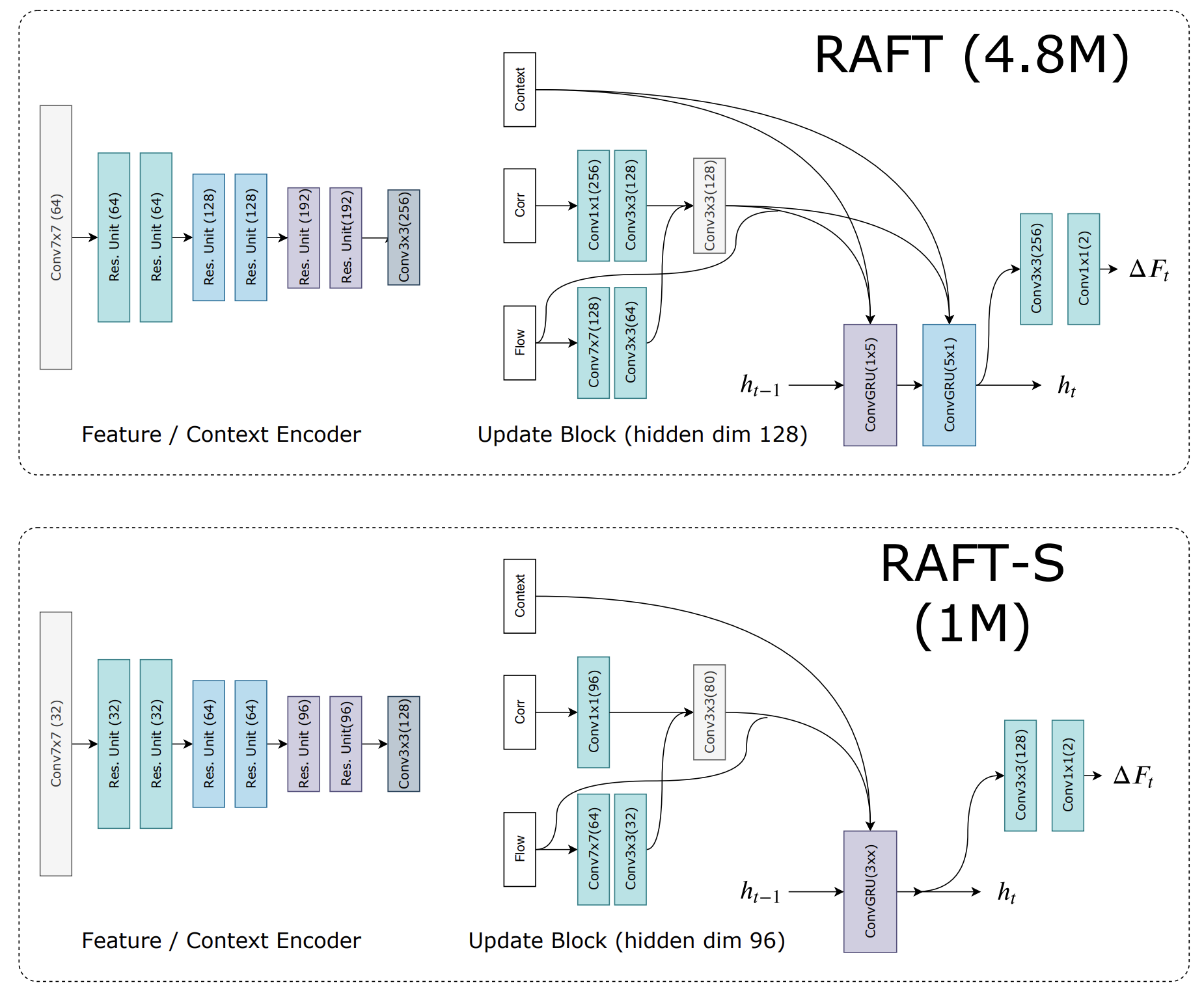
The Feature Encoder module gθ converts the analyzed data into dense feature maps with reduced resolution. In the original version, this resolution is ¹/8 of the original, and the feature dimension D is 256. The encoder consists of six blocks with residual connections, with two convolutional layers at each level. In the context of financial time series, this makes it possible to identify patterns across different time scales: short-term spikes, medium-term trends, and long-term tendencies. This multi-level processing enables the model to see the market as a whole, rather than just individual events.

The hθ context model extracts features only from the first time window (analogous to the first image), ensuring a stable and consistent representation of the data. In trading, this corresponds to an initial assessment of the market state: building a map of relationships between instruments, identifying correlations and hidden signals before iterative forecast refinement begins. Together, the models gθ and hθ form the model's foundation; it is executed once but defines the structure for subsequent updates.

This approach offers a clear advantage over traditional forecasting methods. Instead of relying on a one-off prediction based on past price values, the model creates a rich representation of the market, which is then used for sequential forecast refinement. Each new update takes the entire map of relationships into account and allows the initial estimate to be adjusted, which is especially important in volatile and noisy markets. The resulting architecture turns forecasting not merely into outputting the next value, but into a dynamic reconstruction of the market state that takes many factors into account. This makes it significantly more robust and accurate compared with classic algorithms.

In the next step of the RAFT algorithm, correspondences between features are computed; in the original problem, this is referred to as visual similarity. For financial data, this stage can be interpreted as an assessment of the degree of consistency between time windows and various instruments. In the original architecture, a full correlation field is constructed between all pairs of elements in the two images: C(gθ(I1), gθ(I2)) ∈ R^H×W×H×W, where each correlation cell is a dot product of feature vectors. In the financial interpretation, this can be understood as computing a complete matrix of mutual influence between all points of the time series, making it possible to identify which elements of the previous window have the greatest effect on the forecast values.

To improve efficiency and account for changes at different scales, a four-level correlation pyramid {C1, C2, C3, C4} is constructed, with downsampling pooling (pooling) performed along the last two dimensions at each level using different kernels and strides. This approach provides both high resolution of local interactions and the ability to account for large displacements in the data. In a financial setting, this is analogous to assessing short-term impulses and long-term trends while preserving information about small, rapid price movements that are often critical for an accurate forecast.

The Lookup LC operator is used to retrieve information from the pyramid. It forms a feature map by indexing correlation values based on the current displacement estimates (f1, f2). For each point in the first data window, a correspondence is determined in the next window, after which a local grid with radius r is created around the assumed position. Values from the correlation volume are taken from this grid using bilinear interpolation. This method allows the model to flexibly adjust the forecast by relying on the nearest context and accounting for both point-specific and broader dependencies. In financial data, this corresponds to a weighted assessment of the influence of neighboring points in the time series and related instruments on the current forecast iteration, ensuring resilience to noise and minor anomalies.

All information from every level of the pyramid is consolidated into a single feature map, which is then passed on to the iterative forecast refinement stage. Thus, the correspondence calculation stage provides a rich, multi-level foundation for subsequent analysis, allowing the RAFT model to operate not superficially but systematically, taking into account the full field of interrelationships, which in financial terms corresponds to a deeper understanding of market structure and the dynamics of financial instruments.

The authors of the RAFT framework place particular emphasis on computational efficiency when working with high-dimensional data. The full field of correlations has quadratic complexity O(N²), where N is the number of elements in the window being analyzed. However, it is calculated only once and does not depend on the number of forecast refinement iterations. Furthermore, there is an alternative implementation with linear complexity O(NM) that takes advantage of the linearity of the dot product and preliminary feature averaging. Instead of precomputing the full correlation volume, pyramidal feature representations are formed using downsampling pooling, and the required correlation values are calculated on the fly, only at lookup time.

For financial time series, this type of optimization is critically important. It makes it possible to scale the model to tens or hundreds of assets, work with high-frequency data, and preserve the detail of local movements. Pooling across different time scales can be interpreted as mechanisms for aggregating micro-, meso-, and macro-trends. Dynamic calculation of correlations at query time ensures adaptation to the current market state without the need to store the entire volume of intermediate calculations.

The authors emphasize that even complete precomputation of correlations is not a bottleneck with modern graphics accelerators. In the context of financial models, this means that we are free to choose our strategy: either the most accurate possible modeling of the global field of relationships, or a more economical and adaptive option with dynamic construction of correlations during the iterative process. Both approaches fit seamlessly into the RAFT architecture and allow the model to be applied to market problems without compromising either speed or depth of analysis.

The next stage is the iterative update cycle, in which RAFT evolves from a simple feature-matching model into a full-fledged mechanism for continuous analysis and optimization. At this stage, the system no longer relies on a static correspondence between two fixed market states, but instead treats the forecast as a living hypothesis that must be tested and refined in real time. Each iteration uses not only the current representation of displacement, but also the accumulated hidden context — the internal state. An analog of cognitive memory through which the model tracks the stability of observed interrelationships and the degree of confidence in the current trajectory of capital flows. If new information confirms the previously identified phase structure, the hypothesis is strengthened. If discrepancies are detected, the trajectory is adaptively adjusted. This is no longer just a simple iteration in the code, but a strategic cycle that mimics the behavior of an experienced trader who constantly cross-checks current positions against the changing market picture.

Architecturally, the process is implemented using a recurrent block that is functionally similar to a GRU but adapted to process a spatiotemporal feature field. It takes as input the current correlation features, displacement estimates, and the previous hidden state, generating an update ∆f and an updated internal state. This module links the analytical component (interpreting relationships between features, identifying patterns) with the engineering component (convolution operations, bounded activations, tied weights), ensuring stable convergence to a fixed point, similar to an optimization trajectory. Using convolutional GRU blocks instead of classic fully connected layers expands the local context, allowing the model to account for spatial correlations across multiple scales simultaneously without an excessive increase in the number of parameters.

After each step, the hidden state passes through convolutional layers, generating a flow update ∆f, which is carefully added to the current forecast. At the intermediate stage, the flow is predicted at a reduced resolution of ¹/8. The final step in RAFT is to restore the flow to full scale and refine the mask for each pixel. In a financial context, this is akin to combining micro- and macro-indicators into a single strategic assessment of the market. After generating an update at a lower resolution, the network applies a trainable mask that combines neighboring values in a weighted manner in a 3×3 grid, correcting local errors and improving forecast consistency. Two convolutional layers form a mask of size ^H/8×^W/8×(8×8×9), after which SoftMax is applied, allowing each pixel to take into account the contributions of its neighbors. As a result, the flow prediction becomes smooth, stable, and extremely accurate.

In terms of financial data, this can be viewed as combining short-term liquidity micro-signals with long-term trends and macro indicators. Each local update to the mask adapts the forecast to specific market conditions, eliminating noise and random fluctuations while preserving the global strategic logic of capital movement. This mechanism ensures continuous adaptation, in which micro-level anomalies are corrected without disrupting macro-level navigation through trends and phases of the market cycle.

The use of a trainable mask and upsampling is similar to how an experienced trader combines short-term data with historical context. Each local correction is evaluated in light of the overall market picture and the current position management strategy. This enables RAFT to generate highly accurate forecasts of asset movements, taking into account current micro-impulses and structural macro-patterns, thereby creating a comprehensive, strategically aligned view of the market that is ready for further decision-making and risk modeling.

This provides a fundamental basis for the application of RAFT in financial markets. Instead of taking a deterministic step forward, the model is able to construct a trajectory of the market's probable development, refining it at each stage. This adaptive, dynamic process makes the method particularly valuable in highly volatile environments, where static forecasts quickly become outdated.

An illustration of the RAFT framework, created by the author, is shown below.

Implementation Using MQL5

After reviewing the theoretical aspects of the RAFT framework, we move on to the applied part of our work. At this stage, we are interested not in an abstract concept, but in its practical feasibility within a real trading environment. In this section, we will present one possible way to reproduce the proposed architecture using MQL5 — an environment designed for high-frequency analysis, direct connectivity to liquidity, and strict latency requirements.

This will allow us to verify the correctness of the model and its compatibility with market constraints: order-book update speed, response to volatility spikes, and robustness to local noise. The implementation in MQL5 serves as a kind of stress test for the RAFT framework, demonstrating whether it can operate in systems that make decisions on real data in real time.

In addition, RAFT integrates naturally with risk management tasks. An iterative sequence of forecasts yields not a single value, but a trajectory and a measure of consistency. It can be used to build a probabilistic confidence estimate, adjust position size, and dynamically manage the stop-loss. If the refinements converge quickly and stably, this is a positive signal to increase exposure. If the sequence “jumps” and does not converge, this is a signal to reduce the size or to avoid entering the trade altogether.

However, before moving on to implementation, it is important to understand at a conceptual level how to correctly transfer the ideas of RAFT to the analysis of financial time series. Visual data for optical flow are formed on a two-dimensional coordinate grid, where each pixel has a horizontal and vertical position. Financial features, on the other hand, are a one-dimensional sequence of values over time. Theoretically, it is possible to extend this sequence to a two-dimensional representation, for example by adding a dimension for alternative instruments. But the fundamental difference remains: in an image, a point can move along both axes, including diagonals, which literally means a transfer of energy between adjacent coordinates.

In financial data, nothing flows between features — they cannot migrate between instruments, but only change in value over time. This requires a different way of interpreting spatiotemporal matching, where instead of coordinate displacement we work with the dynamics of values and their local deviations relative to the historical context.

Any adaptation to financial time series must begin with a clear understanding of the economic meaning of each operation. In the original RAFT, the update block is interpreted as an optimization step over the displacement field. In our problems, it becomes a step for re-evaluating the probabilistic market trajectory. This is the key point: the hidden state no longer stores features, but encodes the current degree of confidence in the hypothesis, the risk assessment, and the direction of capital’s internal momentum. Our goal is for each refinement step to yield not only a mathematically consistent improvement in the forecast, but also an economically interpretable adjustment to the position.

Let’s start with the input data format. In the financial version, we treat flow as a vector of forecast increments for each instrument and horizon. This is not a displacement in space, but an increment in expectations: how strongly and in what direction. Correlation features provide a map of consistency — which instruments and which time lags confirm the current hypothesis, and which refute it. The Context vector accumulates macro-level information: volatility, volumes, spreads, and other proxy indicators of the market state. Together, they form the field input to the update block.

Now let’s discuss the update logic itself. It is based on a GRU-like mechanism: the update gate controls how much the model retains its previous position (position inertia), while the reset gate is responsible for the model’s readiness to discard the old hypothesis when there is a strong conflict among features (regime switch). A nonlinear transformation of the hidden state generates a new hypothesis, and then a separate head converts it into a specific expectation increment ∆f. Bounded activations and tied weights act as a controller. They prevent the correction from growing exponentially in the presence of noise and promote convergence to a fixed point, which can be interpreted economically as the attainment of a consensus forecast.

A financial interpretation of architectural techniques is important for decision-making. When the update gate remains close to one, the model demonstrates a consolidation of opinions — confirmation of trend inertia and, consequently, a more aggressive position. If the reset gate is triggered, this signals a possible regime shift: risks are rising, and the model recommends caution, reducing the lot size, or moving to a neutral position. This internal trust-but-verify logic gives the trader an explainable rationale for adjusting exposure and turns the model into a management tool.

A closer examination of the practical side of the approaches proposed by the authors of the RAFT framework reveals a certain similarity to the previously discussed STE-FlowNet framework. And that is not surprising. Both frameworks were originally developed to estimate visual flow and are based on the concept of iterative forecast refinement. In both cases, state correlation and a convolutional GRU block are used, which makes it possible to carefully accumulate information about motion and context. This similarity offers a clear advantage: we can leverage existing work on architecture implementation, computational optimization, and organizing the hidden state, adapting it to financial time series and the specific requirements of working in MQL5. This approach reduces the complexity of implementation, speeds up prototyping, and makes RAFT integration safer and more predictable from both an engineering and economic standpoint.

However, the difference between the approaches is also impossible to ignore. STE-FlowNet uses a U-shaped Encoder-Decoder architecture, in which information is sequentially compressed and then reconstructed to predict the flow. This makes it possible to combine local and global features through skip connections. In contrast, RAFT operates primarily at high resolution and uses correlation map aggregation to create a pyramid that preserves detailed information about each pixel (or feature), while allowing both large and small displacements to be taken into account. This approach makes RAFT more suitable for iterative forecast refinement, especially when high accuracy and the preservation of local data structure are required — which is critical for financial time series, where each data point carries distinct economic significance.

Therefore, we cannot do without refining the existing solutions. And we will start by constructing a feature correlation map. As a baseline option, we can use an existing solution developed as part of the work on the STE-FlowNet framework. As before, instead of a fixed initial state, we will use a stack of the most recent states of the system under analysis. This makes it possible to track not only the current feature values, but also the overall dynamics of changes in the system over time. This approach establishes a historical foundation for iterative forecast refinement, creating a context that takes into account trends, inertia, and short-term market fluctuations — similar to how RAFT, in the visual task of optical flow, detects object motion by taking previous states into account.

However, we need to add the correlation map scaling proposed by the framework's authors. There is a fundamental difference here: in the original RAFT, scaling is performed along the coordinate plane, which makes it possible to track large displacements of objects. This approach cannot be applied to financial time series. An impulse does not move between features, and there is no coordinate grid. Therefore, we shift the scaling to the time axis, allowing the system to track larger impulses in feature changes and their dynamics. This approach preserves the idea of multilevel analysis, similar to a correlation pyramid, but adapted to the economic interpretation of data, where it is important to see both short-term and long-term market changes.

Similarly to the alternative method for computing correlations proposed by the authors, we organize the construction of a multiscale feature map of the state under analysis. First, the map is generated at different time scales, allowing the system to capture both short-term fluctuations and long-term trends. Only then is the overall tensor of aggregated features added to the extended state stack, ensuring data consistency.

We move from the concept of multiscale aggregation to a concrete implementation in an OpenCL kernel, striving to preserve the flow of logic as much as possible. We assume that each work-item / thread is responsible for a specific pair of a feature and the variable being analyzed, and its task is to compute all levels of the time pyramid from this single point, starting from the current value,

and gradually incorporating increasingly deeper history from the stack.

__kernel void AggregationByTime(__global const float* inputs,
                                __global const float* stack,
                                __global float* outputs,
                                const int stack_size,
                                const int levels
                               )
  {
   const size_t id = get_global_id(0);
   const size_t var = get_global_id(1);
   const size_t dimension = get_global_size(0);
   const size_t variables = get_global_size(1);

The kernel algorithm begins by obtaining the feature and variable indices for the current work-item / thread. This allows each time slice and each variable to be processed independently. We read the grid dimensions using get_global_size, fixing the overall dimensionality of the problem space.

The first step is to read the current feature value from the input array inputs. Before writing it, we wrap it with the IsNaNOrInf function to filter out possible artifacts such as NaN or infinity. The resulting value is written to the output array outputs as level zero — this is the freshest state of the system, the reference point for further pyramidal aggregation.

   const float val = IsNaNOrInf(inputs[RCtoFlat(var, id, variables, dimension, 0)], 0);
   outputs[RCtoFlat(var, id, variables, dimension, 0)] = val;

Next, a loop over the levels is started. Each subsequent level l covers twice as many time steps — the block structure is formed according to a power-of-two pattern: 1, 2, 4, 8, and so on. Before adding a new contribution, we attenuate the value of the previously accumulated result by dividing it by two. This is a deliberate exponential decay strategy: this way, we do not recalculate the entire history from scratch, but only adjust the previous aggregation each time to account for the new portion of data.

   for(int l = 1; l < levels; l++)
     {
      int total = pow(2, l);
      int start = total - 1;
      val /= 2;

For level l, we compute the block size as 2 to the power of l and the offset index from the beginning of the stack, from which the current history block is sampled. The nested loop iterates over the elements of the block, but before each iteration we check that we are not going beyond stack_size. This is especially important at the beginning of operation, when the stack depth may still be insufficient.

      for(int s = 0; s < total; s++)
        {
         if(s + start >= stack_size)
            continue;
         val += IsNaNOrInf(stack[RCtoFlat(var, id, variables * levels,
                                          dimension, start + s)] / total, 0);
        }
      outputs[RCtoFlat(var, id, variables, dimension, l)] = IsNaNOrInf(val, 0);
     }
  }

Each historical value is also passed through IsNaNOrInf, then averaged by dividing it by the block size, and added to the already attenuated val.

After processing the block, we store the resulting aggregated value in outputs at the position of the current level l. Thus, each level represents an increasingly generalized picture of the system's dynamics — from an instantaneous reaction to a smoothed response over longer time scales.

The loop structure is completed, and by the time we exit the kernel, the output array contains a fully formed temporal pyramid for the given variable-feature pair, ready for further construction of a multidimensional feature map or for input into the correlation analysis module.

We received a large amount of new information today, and it is clear that we need to give it some time to settle. Let's take a short break to calmly reflect on the material and look at it with fresh eyes. In the next article, we will continue our work with renewed energy and a clearer sense of direction.

Conclusion

In this article, we have come right up to porting the fundamentally powerful RAFT framework to the financial context — and this is precisely where its main advantage becomes apparent. Unlike traditional models, which operate statically and without iterative refinement, RAFT constructs a forecast as a process of continuously approximating the most reliable market trajectory, drawing on multiscale correlation memory. This makes it possible not merely to record price movement, but to track its causal-systemic dynamics, reacting instantly to weak signals before they turn into an explicit trend. This approach paves the way for a new generation of adaptive trading systems — systems capable not of guessing the market, but of methodically narrowing the probability space around its true trajectory.

Links

• RAFT: Recurrent All-Pairs Field Transforms for Optical Flow
• Other articles in this series

Programs used in this article

#	Name	Type	Description
1	Study.mq5	Expert Advisor	Expert Advisor for offline model training
2	StudyOnline.mq5	Expert Advisor	Expert Advisor for online model training
3	Test.mq5	Expert Advisor	Model testing Expert Advisor
4	Trajectory.mqh	Class Library	Structure describing the system state and model architecture
5	NeuroNet.mqh	Class Library	Class library for building a neural network
6	NeuroNet.cl	Library	Code library for the OpenCL program