The MQL5 Standard Library Explorer (Part 15): Building a Market-Regime Classifier with dataanalysis.mqh

In Part 14 of the MQL5 Standard Library Explorer, we moved beyond conventional indicator calculations and used the ALGLIB infrastructure to solve multivariate trading problems. Polynomial regression, rolling correlation analysis, and adaptive hedge estimation demonstrated how mathematical tools can be integrated into complete trading systems. That foundation leads naturally to a larger question: once we have several measurements describing the market, can MetaTrader 5 analyze their combined structure and learn useful distinctions between market states?

This is where dataanalysis.mqh becomes important.

This file is one of the largest components in the MQL5 ALGLIB port. It brings together algorithms for preprocessing, classification, regression, clustering, dimensionality reduction, neural networks, time-series analysis, and nearest-neighbor methods. Rather than studying all of these algorithms as isolated mathematical demonstrations, we will approach the library from the perspective of an algorithmic trader.

Our objective is to build a structured dataset from market bars. We will normalize the variables, inspect structure with Principal Component Analysis (PCA), and train a decision forest to classify each observation by the next completed bar's close-to-close return:

• bearish movement,
• neutral movement,
• bullish movement.

In this article, regime is shorthand for one of these next-close directional classes; it does not mean a complete trend, range, or volatility regime. The important lesson is not that a random forest can predict every next close. It cannot. The purpose is to show how dataanalysis.mqh supports a self-contained training and analysis pipeline in MQL5. The script demonstrates preprocessing, Principal Component Analysis, model fitting, and diagnostics; it is not presented as a production pipeline with chronological validation, model persistence, or live inference.

Contents

1. Understanding dataanalysis.mqh
2. From Price Bars to a Data-Analysis Problem
3. Building the Feature Matrix
4. Normalization with CBdSS
5. Exploring the Feature Space with PCA
6. Building the Decision Forest
7. Making Classifications
8. Evaluating Out-of-Bag Error
9. Variable Importance
10. Completing the Script
11. Designing a Future Trading Component
12. How PCA Complements Decision-Forest Analysis
13. Where k-means++ Fits
14. Testing and Interpretation
15. Important Limitations: Classification Is Not a Trading Edge
16. What dataanalysis.mqh Adds to MQL5 Development
17. Conclusion
18. Table of Attachments

Understanding dataanalysis.mqh

The name dataanalysis.mqh is modest compared with the amount of functionality contained inside it. The file forms the data-analysis layer of the ALGLIB implementation supplied with MetaTrader 5.

Among its important groups are:

The class names below link to the official MetaQuotes ALGLIB package page, which documents the dataanalysis.mqh component and enumerates its data-analysis classes.

Class or component	Purpose	Possible trading application
CBdSS	Dataset normalization, error accumulation, splitting and supporting data-analysis routines	Feature preprocessing and evaluation
CDForest	Decision forests for classification and regression	Market-state classification and nonlinear prediction
CKMeans	k-means++ clustering	Unsupervised market-regime discovery
CLDA	Linear Discriminant Analysis	Separating predefined trading states
CLinReg	Linear regression	Return, spread, volatility, and relationship modeling
CMLPBase / CMLPTrain	Multilayer perceptrons and their training	Nonlinear prediction and classification
CLogit	Multinomial logistic regression	Probability-based directional classification
CPCAnalysis	Principal Component Analysis	Feature compression and factor discovery
CClustering	General clustering framework	Regime discovery and similarity analysis
CSSA	Singular Spectrum Analysis	Trend/noise decomposition and forecasting
CKNN	Nearest-neighbor models	Finding historical market states similar to the current one

This broadens how we can use the Standard Library. We are no longer limited to asking whether RSI crossed 70 or whether two moving averages crossed. We can describe every bar with several measurements and allow a statistical model to study their relationship to an outcome.

From Price Bars to a Data-Analysis Problem

A machine-learning algorithm does not understand candles, trends, support levels, or market psychology in the way a trader describes them. It receives numbers.

We therefore begin by translating each historical observation into a row of variables.

For this experiment, each observation contains five features:

Feature	Description
Return1	One-bar relative return from the previous close
BodyRatio	Signed candle body, (close - open), divided by the high-low range
RangeRatio	High-low range relative to closing price
Momentum3	Three-bar relative return
Momentum10	Ten-bar relative return

The sixth column is not an input variable; it stores the class label.

We define the class from the next completed bar's close-to-close relative return:

• class 0 = bearish,
• class 1 = neutral,
• class 2 = bullish.

A configurable threshold prevents very small movements from being treated as meaningful directional events.

Conceptually, each training row therefore looks like this:

Return1 | BodyRatio | RangeRatio | Momentum3 | Momentum10 | Class

This structure matches an important convention used by the decision-forest routines: independent variables occupy the first columns, while the final column contains the class identifier for a classification problem.

Building the Feature Matrix

The first implementation is a script called MarketRegimeForest.mq5. It downloads historical bars, constructs the dataset, trains the model, and displays the resulting diagnostics.

//+------------------------------------------------------------------+
//|                                          MarketRegimeForest.mq5  |
//|                                Copyright 2026, Clemence Benjamin |
//|                                         https://www.mql5.com     |
//+------------------------------------------------------------------+
#property copyright "Copyright 2026, Clemence Benjamin"
#property version   "1.00"
#property strict

//--- Include the ALGLIB data analysis library (decision forest, PCA, etc.)
#include <Math\Alglib\dataanalysis.mqh>

//--- Input parameters
input int      InpBars             = 1500;    // Number of history bars used for training
input int      InpTrees            = 100;     // Number of trees in the random forest
input double   InpNeutralThreshold = 0.00050; // Return threshold defining the neutral regime
input int      InpSeed             = 2026;    // Random seed for reproducible training

//--- Model configuration constants
#define FEATURES 5   // Number of predictive features per sample
#define CLASSES  3   // Number of target classes: 0-Bearish, 1-Neutral, 2-Bullish

We use ordinary price information so that the data-analysis process remains visible. Indicator handles can be introduced later without changing the model-building principles.

//+------------------------------------------------------------------+
//| Classifies a future return into a market regime class            |
//| Returns: 0 - bearish, 1 - neutral, 2 - bullish                   |
//+------------------------------------------------------------------+
int DirectionClass(const double future_return)
  {
   if(future_return<-InpNeutralThreshold)
      return(0);   // Significant negative move -> bearish regime
   if(future_return>InpNeutralThreshold)
      return(2);   // Significant positive move -> bullish regime
   return(1);      // Small move -> neutral regime
  }

The feature-building routine converts the price series into a matrix.

//+------------------------------------------------------------------+
//| Builds the labeled training dataset from price history           |
//| Computes the feature vectors and their future-return class labels|
//+------------------------------------------------------------------+
bool BuildDataset(MqlRates &rates[],const int total,CMatrixDouble &xy,int &samples)
  {
   const int first=10;            // Skip bars needed for the momentum look-back
   const int last=total-2;        // Keep one future bar for label computation
   if(last<=first)
      return(false);              // Not enough data to build the dataset

   samples=last-first+1;
   xy.Resize(samples,FEATURES+1);
   int row=0;

   for(int i=first;i<=last;i++)
     {
      double prev_close=rates[i-1].close;
      //--- Reject division by zero or invalid prices
      if(prev_close==0.0 ||
         rates[i-3].close==0.0 ||
         rates[i-10].close==0.0 ||
         rates[i].close==0.0)
         return(false);

      //--- Candle-derived features
      double candle_range=rates[i].high-rates[i].low;               // High-Low range
      double return1=(rates[i].close-prev_close)/prev_close;        // 1-bar return
      double body_ratio=0.0;

      //--- Body ratio: signed candle body divided by the candle range
      if(candle_range>0.0)
         body_ratio=(rates[i].close-rates[i].open)/candle_range;

      double range_ratio=candle_range/rates[i].close;               // Normalized volatility
      double momentum3=(rates[i].close-rates[i-3].close)/rates[i-3].close;   // 3-bar momentum
      double momentum10=(rates[i].close-rates[i-10].close)/rates[i-10].close; // 10-bar momentum

      //--- Target label: next completed bar's close-to-close return
      double future_return=(rates[i+1].close-rates[i].close)/rates[i].close;

      //--- Store the feature vector
      xy.Set(row,0,return1);
      xy.Set(row,1,body_ratio);
      xy.Set(row,2,range_ratio);
      xy.Set(row,3,momentum3);
      xy.Set(row,4,momentum10);
      //--- Store the class label (last column)
      xy.Set(row,5,DirectionClass(future_return));
      row++;
     }

   return(true);
  }

Notice that the target is separated in time from the features. Data from bar i forms the model input, while the close-to-close return from bar i to completed bar i+1 determines the label. The label describes the change between two closes; it does not encode the next candle's complete OHLC path.

This separation is fundamental. If future information leaks into the input features, the accuracy becomes meaningless because the model learns from data unavailable in real trading.

Normalization with CBdSS

One of the first components in dataanalysis.mqh is CBdSS. Its DSNormalize and DSNormalizeC routines calculate variable means and standard deviations, while DSNormalize additionally standardizes the feature matrix.

For a variable x, standardization follows the familiar transformation:

z = (x - mean) / sigma

where z is the standardized feature value, x is the original feature value, mean is the training-sample mean of that feature, and sigma is its training-sample standard deviation.

This places variables measured on different scales into a comparable numerical space.

For our dataset we must normalize only the five independent variables. Class labels must remain integers from 0 to 2.

//+------------------------------------------------------------------+
//| Normalizes features to zero mean and unit variance (z-score)     |
//+------------------------------------------------------------------+
bool NormalizeFeatures(CMatrixDouble &xy,const int samples,double &means[],double &sigmas[])
  {
   CMatrixDouble features;
   features.Resize(samples,FEATURES);

//--- Copy the feature columns into a separate matrix
   for(int i=0;i<samples;i++)
      for(int j=0;j<FEATURES;j++)
         features.Set(i,j,xy.Get(i,j));

//--- Perform z-score normalization using ALGLIB
   int info=0;
   CBdSS::DSNormalize(features,samples,FEATURES,info,means,sigmas);

   if(info!=1)
     {
      Print("DSNormalize failed. Info=",info);
      return(false);
     }

//--- Write the normalized features back into the dataset
   for(int i=0;i<samples;i++)
      for(int j=0;j<FEATURES;j++)
         xy.Set(i,j,features.Get(i,j));

   return(true);
  }

The means and standard deviations are retained because live observations must later undergo exactly the same transformation used for the training data.

Recalculating a different mean and standard deviation for every incoming observation would change the coordinate system seen by the model. If a stored sigma is zero, production code should explicitly set that standardized feature to zero or reject it; the compact helper shown here leaves such a feature unchanged.

Exploring the Feature Space with PCA

Before training the classifier, we can examine whether our five variables actually represent five independent dimensions of information.

CPCAnalysis provides Principal Component Analysis.

PCA rotates the original feature space into orthogonal directions ordered by the amount of variance they explain. If the first two components explain most of the dataset's variation, several of our original features may be strongly related.

We first copy only the feature columns:

//+------------------------------------------------------------------+
//| Runs Principal Component Analysis and reports variance shares    |
//+------------------------------------------------------------------+
void AnalyzePCA(CMatrixDouble &xy,const int samples)
  {
   CMatrixDouble features;
   features.Resize(samples,FEATURES);

//--- Copy the feature columns for PCA analysis
   for(int i=0;i<samples;i++)
      for(int j=0;j<FEATURES;j++)
         features.Set(i,j,xy.Get(i,j));

//--- Build the PCA basis using ALGLIB
   int info=0;
   double variance[];
   CMatrixDouble basis;

   CPCAnalysis::PCABuildBasis(features,samples,FEATURES,info,variance,basis);

   if(info!=1)
     {
      Print("PCA failed. Info=",info);
      return;
     }

//--- Compute the total variance for share calculation
   double total=0.0;
   for(int i=0;i<ArraySize(variance);i++)
      total+=variance[i];

   Print("----- PCA -----");
   double cumulative=0.0;

//--- Report the explained variance of each principal component
   for(int i=0;i<ArraySize(variance);i++)
     {
      double share=0.0;
      if(total>0.0)
         share=variance[i]/total;

      cumulative+=share;
      PrintFormat("PC%d variance share = %.2f%% | cumulative = %.2f%%",
                  i+1,100.0*share,100.0*cumulative);
     }
  }

PCA is not being used here as a magic predictor. Its role is diagnostic.

If Return1, Momentum3, and Momentum10 all describe closely related directional information, PCA should expose that redundancy. We can then decide whether to retain all variables, remove some, or eventually train another model using principal-component scores instead of the original features.

This is one of the benefits of examining data structure before concentrating on trading signals.

Building the Decision Forest

The central model of this experiment is CDForest.

A single decision tree repeatedly divides observations according to feature thresholds. CDForest is a decision-forest implementation, and DFBuilderBuildRandomForest() configures it as a random forest by using randomized observations and candidate variables. Their combined output is generally more stable than that of one tree.

The implementation exposes a builder-oriented workflow:

1. Create a CDecisionForestBuilder.
2. Assign the dataset.
3. Configure random-variable selection and subsampling.
4. Configure variable importance.
5. Set a reproducible seed if required.
6. Build the requested number of trees.

The model objects are declared globally:

//--- Global objects of the decision forest model
CDecisionForestBuilder g_builder;   // Builder used to construct the forest
CDecisionForest        g_forest;    // Trained random forest model
CDFReport              g_report;    // Training report (errors, variable importance)

//--- Feature normalization statistics (z-score scaling)
double g_means[];    // Mean of each feature
double g_sigmas[];   // Standard deviation of each feature

The training function is compact because most of the algorithmic complexity already exists inside dataanalysis.mqh.

//+------------------------------------------------------------------+
//| Trains the random forest classifier on the prepared dataset      |
//+------------------------------------------------------------------+
bool TrainForest(CMatrixDouble &xy,const int samples)
  {
//--- Create and configure the decision forest builder
   CDForest::DFBuilderCreate(g_builder);
   CDForest::DFBuilderSetDataset(g_builder,xy,samples,FEATURES,CLASSES);
   CDForest::DFBuilderSetRndVarsAuto(g_builder);           // Auto-select random variables
   CDForest::DFBuilderSetSubsampleRatio(g_builder,0.50);   // Use 50% of samples per tree
   CDForest::DFBuilderSetSeed(g_builder,InpSeed);          // Reproducibility
   CDForest::DFBuilderSetImportancePermutation(g_builder); // Enable permutation importance

//--- Build the random forest model
   CDForest::DFBuilderBuildRandomForest(g_builder,InpTrees,g_forest,g_report);
   return(true);
  }

Several details deserve attention.

• DFBuilderSetRndVarsAuto() leaves selection of the number of randomly considered variables to the forest builder.
• DFBuilderSetSubsampleRatio() controls the fraction of observations selected when individual trees are created.
• DFBuilderSetSeed() is particularly important while developing an article or debugging a strategy. A positive fixed seed makes repeated runs on the same dataset reproducible. Without it, slightly different forests can be produced because of randomized sampling.
• DFBuilderSetImportancePermutation() instructs the builder to calculate permutation-based variable importance. We will use that information later to determine which market measurements contribute most to the classifier.

Making Classifications

Once the forest has been built, a new market observation is simply another vector containing the same five features used during training.

It must first be normalized using the training statistics. PredictClass() expects that preprocessing to have happened already; it does not normalize its argument. The helper demonstrates the inference interface, but OnStart() does not call it in this training-and-diagnostics script. A future EA should wrap normalization and classification in one safe method so that callers cannot accidentally submit raw features.

//+------------------------------------------------------------------+
//| Normalizes a single observation using the training statistics    |
//+------------------------------------------------------------------+
void NormalizeObservation(double &x[])
  {
   for(int j=0;j<FEATURES;j++)
      if(g_sigmas[j]!=0.0)
         x[j]=(x[j]-g_means[j])/g_sigmas[j];
  }

CDForest exposes both classification helpers and lower-level processing routines.

//+------------------------------------------------------------------+
//| Classifies a feature vector and returns the predicted class      |
//+------------------------------------------------------------------+
int PredictClass(double &features[])
  {
   CRowDouble x=features;
   return(CDForest::DFClassify(g_forest,x));
  }

A predicted class can then be translated back into trading language:

//+------------------------------------------------------------------+
//| Returns a human-readable name for a regime class                 |
//+------------------------------------------------------------------+
string RegimeName(const int cls)
  {
   if(cls==0)
      return("BEARISH");
   if(cls==2)
      return("BULLISH");
   return("NEUTRAL");
  }

This transformation is simple, but conceptually important. The forest does not know what bullish means. It only learns the numerical distinctions associated with classes 0, 1, and 2.

Evaluating Out-of-Bag Error

A major advantage of the decision-forest implementation is that its report contains more than a training accuracy number.

CDFReport stores training errors as well as corresponding out-of-bag statistics.

Out-of-bag (OOB) observations are samples that were not selected for a particular tree's training subset. They estimate how the forest behaves on rows excluded from those trees, but they are not an independent chronological out-of-sample test. Consecutive market observations are dependent, and randomized subsampling does not preserve the forward order required for trading validation. OOB diagnostics are useful for comparison, but they cannot replace a holdout period or walk-forward test.

//+------------------------------------------------------------------+
//| Prints the decision forest training report to the journal        |
//+------------------------------------------------------------------+
void PrintForestReport()
  {
   Print("----- DECISION FOREST REPORT -----");
   PrintFormat("Training relative classification error: %.6f",g_report.m_RelCLSError);
   PrintFormat("OOB relative classification error: %.6f",g_report.m_oobrelclserror);
   PrintFormat("Training RMS error: %.6f",g_report.m_RMSError);
   PrintFormat("OOB RMS error: %.6f",g_report.m_oobrmserror);
   PrintFormat("Training average error: %.6f",g_report.m_AvgError);
   PrintFormat("OOB average error: %.6f",g_report.m_oobavgerror);
  }

The difference between training and OOB performance can tell us more than the training number alone.

If training error becomes extremely low while OOB error remains high, the model may be memorizing characteristics of the historical sample that do not generalize well.

For algorithmic trading, this distinction is especially important because financial data are noisy, and market relationships change over time.

Variable Importance

We deliberately selected permutation importance when configuring the builder.

The resulting CDFReport contains:

• m_varimportances — importance ratings,
• m_topvars — feature indices ordered by importance.

We can make these indices readable:

//+------------------------------------------------------------------+
//| Returns the descriptive name of a feature by index               |
//+------------------------------------------------------------------+
string FeatureName(const int index)
  {
   switch(index)
     {
      case 0: return("Return1");     // 1-bar return
      case 1: return("BodyRatio");   // Signed candle body ratio
      case 2: return("RangeRatio");  // Normalized candle range
      case 3: return("Momentum3");   // 3-bar momentum
      case 4: return("Momentum10");  // 10-bar momentum
     }
   return("Unknown");
  }

Then display the rankings:

//+------------------------------------------------------------------+
//| Prints the variable importance ranking to the journal            |
//+------------------------------------------------------------------+
void PrintVariableImportance()
  {
   Print("----- VARIABLE IMPORTANCE -----");
   for(int rank=0;rank<FEATURES;rank++)
     {
      int index=g_report.m_topvars[rank];
      PrintFormat("%d. %s = %.6f",
                  rank+1,
                  FeatureName(index),
                  g_report.m_varimportances[index]);
     }
  }

This is where machine learning becomes useful for research rather than merely prediction.

Suppose Momentum10 consistently ranks first while candle body contributes almost nothing. The result does not prove that Momentum10 is universally superior, but it gives us an empirical reason to investigate the relationship further.

Conversely, if an expensive indicator contributes negligible incremental information, variable-importance analysis may justify removing it from the model.

Completing the Script

The OnStart() routine connects the individual stages.

//+------------------------------------------------------------------+
//| Script entry point: loads history, trains the model, reports     |
//+------------------------------------------------------------------+
void OnStart()
  {
   MqlRates rates[];
   ArraySetAsSeries(rates,false);

//--- Load completed bars and use non-series chronological indexing
   int copied=CopyRates(_Symbol,_Period,1,InpBars,rates);

//--- Ensure enough data is available for training
   if(copied<50)
     {
      Print("Not enough historical bars. Copied=",copied);
      return;
     }

   CMatrixDouble dataset;
   int samples=0;

//--- Build the labeled training dataset
   if(!BuildDataset(rates,copied,dataset,samples))
     {
      Print("Unable to construct dataset.");
      return;
     }

   PrintFormat("Dataset created: %d samples, %d features.",samples,FEATURES);

//--- Normalize features and stop on failure
   if(!NormalizeFeatures(dataset,samples,g_means,g_sigmas))
      return;

//--- Analyze the feature structure with PCA
   AnalyzePCA(dataset,samples);

//--- Train the random forest classifier
   if(!TrainForest(dataset,samples))
      return;

//--- Output the model quality report and feature importance
   PrintForestReport();
   PrintVariableImportance();
   Print("Market regime model completed.");
  }
//+------------------------------------------------------------------+

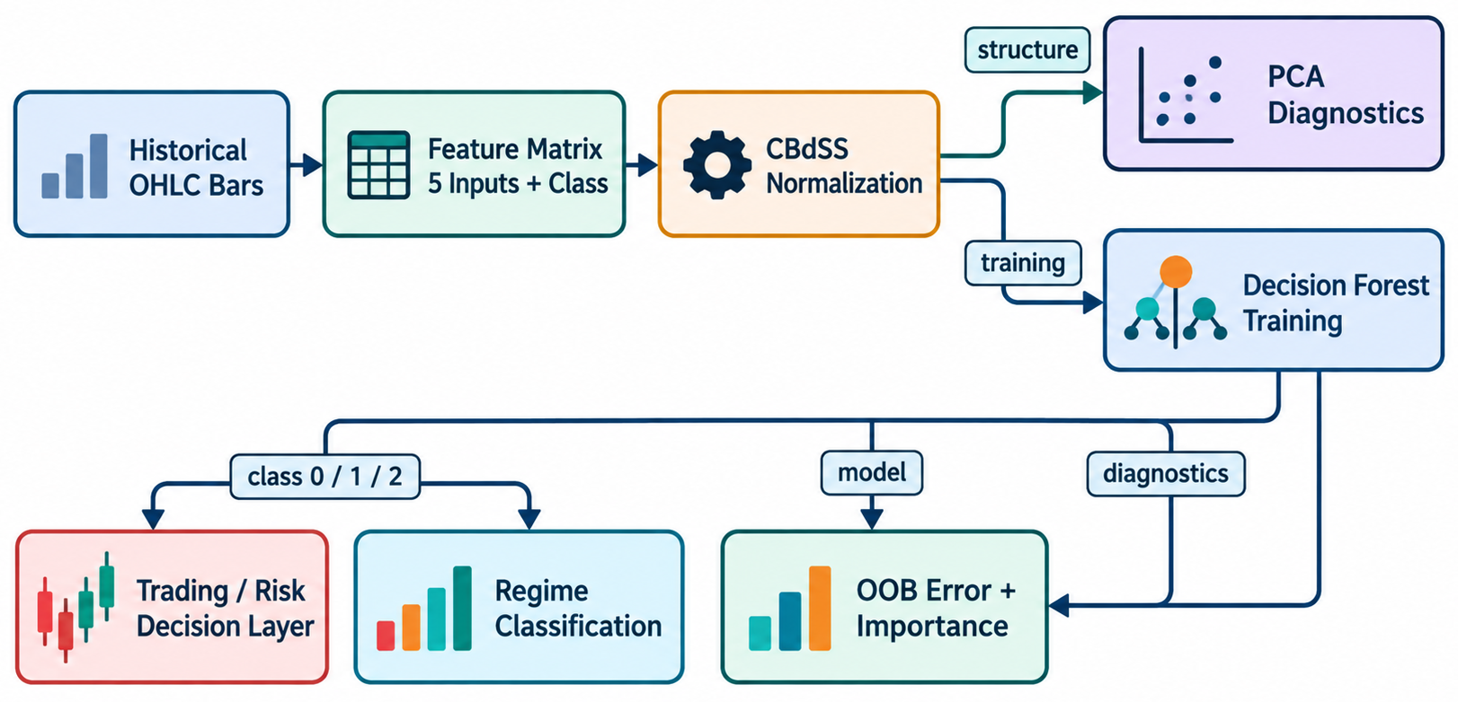
Fig. 1. Market-regime classification pipeline implemented with dataanalysis.mqh.

This is substantially different from an Expert Advisor whose logic consists of a fixed sequence, such as the following:

if(rsi<30 && close>moving_average)
   Buy();

There is nothing inherently wrong with deterministic rules. In fact, they are often preferable when the relationship is simple and well understood. The difference is that dataanalysis.mqh lets us investigate relationships that are difficult to express as one threshold or one crossover.

Designing a Future Trading Component

The current script deliberately stops before order execution. Classification quality must be investigated before a statistical model is allowed to control positions.

Once validated, however, the architecture can be moved into an Expert Advisor.

A practical EA would separate the system into four stages:

Stage	Responsibility
Data preparation	Update market features only after a completed bar
Model	Normalize each observation and obtain its predicted class
Decision layer	Translate classifications into allowable trade states
Execution/risk layer	Apply position sizing, stop-loss rules, spread filters, and order management

The model should therefore not directly call Buy() or Sell().

Instead, it may return:

0 = bearish
1 = neutral
2 = bullish

The trading engine can then decide what those states mean under the current risk policy.

For example, a bullish classification could be ignored when the spread is too large or maximum risk has already been reached. If a future implementation also exposes normalized class scores, the decision layer could add a confidence threshold; the current script returns only the winning class.

How PCA Complements Decision-Forest Analysis

There is an interesting relationship between the two algorithms used in this article.

PCA asks: How is variation structured across our variables?

The decision forest asks: Can combinations of those variables separate the classes we defined?

These are not the same question.

A variable can explain a large amount of overall variance without being strongly predictive of direction. Likewise, a lower-variance feature can still be useful for distinguishing particular market regimes.

For that reason, PCA variance should not be mistaken for predictive importance.

By comparing PCA structure with forest variable importance we obtain two complementary views of the dataset.

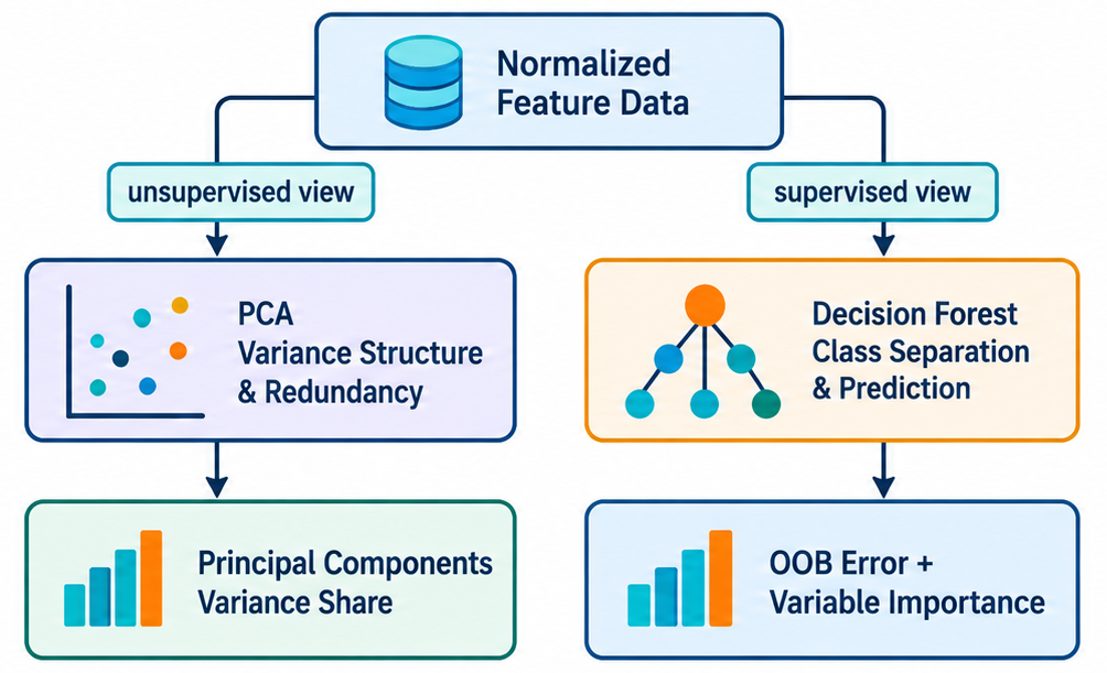
Fig. 2. PCA and decision forests provide complementary views of the same market-feature dataset.

Where k-means++ Fits

The file also implements CKMeans and the larger CClustering framework. These provide an alternative route when we do not want to define bullish, neutral, and bearish classes in advance.

Instead of saying:

future return > threshold = bullish

we can present the market features to a clustering algorithm and ask it to discover natural groups.

One cluster might eventually correspond to high-volatility directional movement, another to quiet consolidation, and another to transitional conditions.

This difference separates two important approaches:

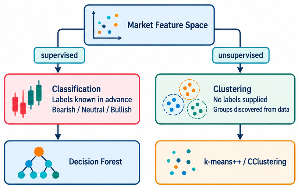
Fig. 3. Classification uses predefined market states, while clustering discovers groups directly from the feature data.

Approach	Question
Classification	Can the model learn classes that we defined?
Clustering	What groups naturally exist in the data?

That distinction creates several possible extensions for the Standard Library Explorer series.

Testing and Interpretation

When the script is executed, the important output is not a single "accuracy" figure.

The current script reports three groups of diagnostics:

• training versus out-of-bag error,
• the PCA variance distribution,
• the ranking of feature importance.

Class distribution should also be inspected before using the model, but this version does not print those counts. Add a class counter or a separate dataset audit before interpreting accuracy under a wide neutral threshold.

A model can appear accurate simply because one class dominates the dataset.

For example, if the neutral threshold is too wide, most observations may become class 1. A classifier that repeatedly predicts "neutral" could then report an apparently respectable result without discovering a useful directional relationship.

This is why dataset construction is at least as important as model selection.

Live Demo Result on EURUSD H1

We ran MarketRegimeForest.mq5 on a live demo EURUSD H1 chart using the default article settings. The resulting decision-forest report showed a training relative classification error of 0.013432 and an out-of-bag relative classification error of 0.337139.

The large difference between these two values is important. The forest fits the training observations very closely, while its error on rows excluded from individual tree-training subsets is considerably higher. This warns us about overfitting, but it is not evidence of forward performance. Because adjacent bar-derived rows are dependent, only a later holdout interval or walk-forward sequence can test chronological generalization.

Metric	Training	Out-of-bag
Relative classification error	0.013432	0.337139
RMS error	0.201457	0.400125
Average error	0.152116	0.303935

Permutation importance produced another useful diagnostic. RangeRatio ranked first, followed by Return1 and Momentum3. BodyRatio and Momentum10 received zero importance in this particular run.

Rank	Feature	Permutation importance
1	RangeRatio	0.035026
2	Return1	0.012249
3	Momentum3	0.007864
4	BodyRatio	0.000000
5	Momentum10	0.000000

The result should not be interpreted as proof that RangeRatio is universally the best predictor or that BodyRatio and Momentum10 are useless. It describes this EURUSD H1 sample under the current settings. Repeating the experiment across different windows, symbols, timeframes, thresholds, and walk-forward periods is necessary before drawing stronger conclusions. We must also fit normalization statistics on each training window and apply them unchanged to its later validation window.

2026.08.14 16:22:41.664 MarketRegimeForest (EURUSD,H1)  ----- DECISION FOREST REPORT -----
2026.08.14 16:22:41.665 MarketRegimeForest (EURUSD,H1)  Training relative classification error: 0.013432
2026.08.14 16:22:41.665 MarketRegimeForest (EURUSD,H1)  OOB relative classification error: 0.337139
2026.08.14 16:22:41.665 MarketRegimeForest (EURUSD,H1)  Training RMS error: 0.201457
2026.08.14 16:22:41.665 MarketRegimeForest (EURUSD,H1)  OOB RMS error: 0.400125
2026.08.14 16:22:41.665 MarketRegimeForest (EURUSD,H1)  Training average error: 0.152116
2026.08.14 16:22:41.665 MarketRegimeForest (EURUSD,H1)  OOB average error: 0.303935
2026.08.14 16:22:41.665 MarketRegimeForest (EURUSD,H1)  ----- VARIABLE IMPORTANCE -----
2026.08.14 16:22:41.665 MarketRegimeForest (EURUSD,H1)  1. RangeRatio = 0.035026
2026.08.14 16:22:41.665 MarketRegimeForest (EURUSD,H1)  2. Return1 = 0.012249
2026.08.14 16:22:41.665 MarketRegimeForest (EURUSD,H1)  3. Momentum3 = 0.007864
2026.08.14 16:22:41.665 MarketRegimeForest (EURUSD,H1)  4. BodyRatio = 0.000000
2026.08.14 16:22:41.665 MarketRegimeForest (EURUSD,H1)  5. Momentum10 = 0.000000
2026.08.14 16:22:41.665 MarketRegimeForest (EURUSD,H1)  Market regime model completed.

Several variables should therefore be tested:

Parameter	Research question
Neutral threshold	How much movement should count as directional?
Training window	Does the relationship persist across different samples?
Number of trees	Does additional ensemble size improve stability?
Subsample ratio	How sensitive is the model to resampling?
Feature set	Which variables add genuine information?
Timeframe	Does the learned structure depend on sampling frequency?

Important Limitations: Classification Is Not a Trading Edge

This compact experiment standardizes the entire dataset before the forest calculates OOB error. Consequently, every row contributes to the means and standard deviations, including rows that are OOB for individual trees. This is a weak form of information leakage in the diagnostic estimate. A stricter experiment must fit normalization on the training window only and apply those stored statistics to a later validation or walk-forward window.

\n

BuildDataset() also treats a zero close as invalid and stops the complete build. That conservative behavior is acceptable for normal broker history, where zero closes should not occur, but a production data pipeline should diagnose or skip damaged rows and verify that the final row count matches the allocated sample count.

\n

A classification model and a profitable trading system are not equivalent.

Even when a classifier detects directional structure, the economic value of that structure still depends on:

• spread,
• commission,
• slippage,
• trade frequency,
• risk-reward characteristics,
• class imbalance,
• regime stability,
• out-of-sample persistence.

A model that predicts tiny movements correctly may have no tradable value after transaction costs.

This is why our implementation deliberately treats data analysis and execution as separate layers.

What dataanalysis.mqh Adds to MQL5 Development

The most important observation from this exploration is architectural.

MetaTrader 5 already provides the infrastructure to move from rule-based strategies to statistical learning, without exporting calculations to Python or another external environment.

Using one Standard Library component we can:

• normalize datasets,
• calculate model errors,
• perform linear and multinomial regression,
• train decision forests,
• build neural networks,
• perform PCA and LDA,
• cluster observations,
• analyze time series with SSA,
• build nearest-neighbor models.

The value for an MQL5 developer is not simply the number of algorithms available. It is the ability to place data acquisition, analysis, model inference, chart visualization, risk management, execution, and Strategy Tester evaluation inside the same development environment.

Conclusion

In Part 14, the ALGLIB port helped us solve numerical problems underlying dynamic hedging. In this part, dataanalysis.mqh moves us from numerical computation into structured data learning.

We constructed a self-contained analytical workflow beginning with ordinary OHLC bars. The bars were transformed into numerical features, standardized through CBdSS, inspected with Principal Component Analysis, and supplied to a decision forest for three-class market-regime classification.

More importantly, we did not stop after fitting the forest. Its report gave us out-of-bag diagnostics and variable-importance information, allowing us to investigate the gap between training fit and resampled diagnostics and to see which variables contributed to that result.

This is the larger lesson of data analysis in algorithmic trading. The objective is not to replace trading logic with a mysterious prediction function. It is to build a measurable chain from raw data to features, from features to models, from models to diagnostics, and only then from diagnostics to trading decisions.

dataanalysis.mqh gives MQL5 developers a comprehensive toolbox for turning market data into interpretable machine-learning workflows. With preprocessing, dimensionality analysis, classification, out-of-bag diagnostics, and variable-importance analysis available within the same environment, developers can study how a model is formed and whether its features contain useful information. Chronological holdout and walk-forward validation remain separate requirements before the model can support trading decisions.

Table of Attachments

The attached script belongs in the Scripts branch of the terminal's MQL5 data folder. The project folder structure used for this article is shown below.

File	Type	Folder structure	Description
MarketRegimeForest.mq5	Script	MQL5\Scripts\StandardLibraryExplorer\Part15\MarketRegimeForest.mq5	Main Part 15 script. It builds the labeled feature matrix, normalizes the predictive variables, performs PCA diagnostics, trains the decision forest, and prints training, out-of-bag, and permutation-importance results to the Journal.