Neural Networks in Trading: Decomposition Instead of Scaling — Building Modules

Introduction

In the previous article, we began working on implementing our own vision of the approaches proposed by the authors of the SSCNN framework. In this article, we will continue by moving on to the practical aspects of implementing the framework's key components. However, before delving into the code and algorithms, it is important to remind the reader of the strengths of SSCNN and how it works. Understanding these fundamentals will allow you not only to replicate the implementation but also to consciously adapt it to real-world trading tasks.

The SSCNN (Segmental Structured Convolutional Neural Network) framework was developed as a specialized tool for analyzing time series under conditions of market instability and fragmented signals. Its central idea is to process not individual values, but complete data segments, allowing the model to take into account both local features and broader contextual dependencies. Instead of a linear view of a time series, SSCNN offers a stratified approach: each time interval is considered within the structure of its surrounding context, making it possible to accurately extract meaningful features even in the presence of a high level of noise.

In the first stage, the data undergo a structural decomposition process, in which the signal is broken down into stable components: a long-term trend, seasonal variations, short-term fluctuations, and residual noise. This step is particularly important when working with financial time series, where trends and short-term deviations carry different analytical significance. Separate processing models are created for each component, which improves the quality of the analysis and the interpretability of the results. The final forecast is built as a coherent aggregation of outputs from these models.

In SSCNN, particular emphasis is placed on the attention-based normalization mechanism (AttnNorm). This component not only stabilizes the model's internal representations but also allows it to adaptively focus on the most informative parts of the data. In conditions of market turbulence, where the signal can be significantly distorted by short-term spikes, this selectivity ensures the stability and accuracy of the forecast. Normalization is implemented with the segmental context taken into account and includes the training of attention parameters, making backpropagation more meaningful and targeted.

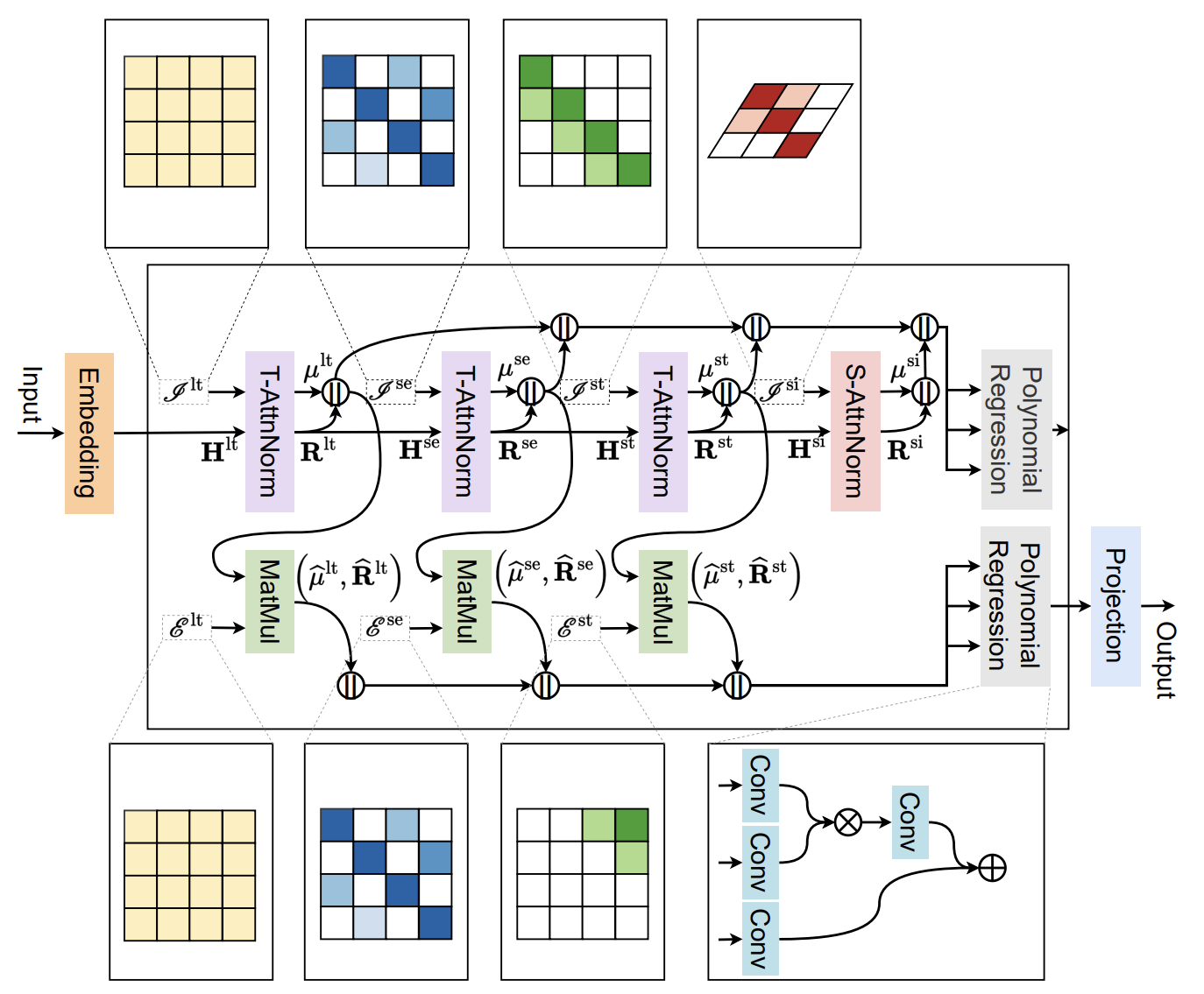
An author-created visualization of the SSCNN framework is shown below.

Component Extraction Module

In the practical section of the previous article, we focused on implementing a normalization kernel with attention weights in the OpenCL environment. This work allowed us to lay the groundwork for the fast, parallel execution of key operations: calculating mean values and standard deviations across data segments while accounting for attention weights, as well as directly normalizing the input signal. All of this is performed within the GPU context, which ensures high performance and scalability of the solution.

Today, we are naturally continuing the work we started earlier and shifting our focus to how the main program interacts with these OpenCL kernels. We need to implement the algorithms for handling them, including buffer preparation, configuration of call parameters, synchronization, and verification of the integrity of the transmitted data. This is an important step: after all, the effectiveness of the SSCNN framework depends largely not only on the mathematical accuracy of the kernel, but also on how competently and coherently data exchange between the CPU and the GPU is organized.

The central element of the design is the CNeuronAttentNorm object. It is responsible for coordinating the interaction between the high-level logic of the attention normalization layer and low-level GPU computation. This object inherits from the base class CNeuronBaseOCL, which provides it with a universal interface and allows it to be integrated into the overall model stack without losing flexibility. The structure of the new object is shown below.

class CNeuronAttentNorm :  public CNeuronBaseOCL
  {
protected:
   uint                    iPeriod;
   uint                    iVariables;
   uint                    iCount;
   //---
   CParams                 cAttention;
   CNeuronSoftMaxOCL       cSoftMax;
   CNeuronBaseOCL          cMeans;
   CNeuronBaseOCL          cSTDevs;
   //---
   virtual bool      AttentNorm(CNeuronBaseOCL *NeuronOCL);
   virtual bool      AttentNormGrad(CNeuronBaseOCL *NeuronOCL);
   //---
   virtual bool      feedForward(CNeuronBaseOCL *NeuronOCL) override;
   virtual bool      updateInputWeights(CNeuronBaseOCL *NeuronOCL) override;
   virtual bool      calcInputGradients(CNeuronBaseOCL *NeuronOCL) override;

public:
                     CNeuronAttentNorm(void) :  iPeriod(0), iVariables(0), iCount(0) {};
                    ~CNeuronAttentNorm(void) {};
   //---
   virtual bool      Init(uint numOutputs, uint myIndex, COpenCLMy *open_cl,
                          uint units_count, uint period, uint variables,
                          ENUM_OPTIMIZATION optimization_type, uint batch);
   //---
   virtual bool      Save(const int file_handle) override;
   virtual bool      Load(const int file_handle) override;
   //---
   virtual int       Type(void) override const  {  return defNeuronAttentNorm; }
   virtual void      SetOpenCL(COpenCLMy *obj) override;
   //---
   CNeuronBaseOCL*   GetMeans(void) { return cMeans.AsObject(); }
   CNeuronBaseOCL*   GetSTDevs(void) { return cSTDevs.AsObject(); }
   virtual uint      GetPeriod(void) const { return iPeriod; }
   virtual uint      GetVariables(void) const { return iVariables; }
   virtual uint      GetUnits(void) const { return iCount; }
   //---
   virtual bool      WeightsUpdate(CNeuronBaseOCL *source, float tau) override;
   virtual void      SetActivationFunction(ENUM_ACTIVATION value) override {  activation = None; }
  };

In the class structure, we can see that the key internal parameters are iPeriod, iVariables, and iCount: they specify the size of the data segment, the number of variables, and the number of segments in a single unit sequence, respectively. These values define the structure of the array being analyzed.

Special attention should be paid to the cAttention object, which stores parameters related to the attention mechanism, and to cSoftMax: the component that converts attention weights into a normalized form. These two modules work in close coordination: the trainable attention parameters undergo a SoftMax transformation, and only then are they used to compute the means and standard deviations. The cMeans and cSTDevs objects are used to store these statistics.

All internal objects of the CNeuronAttentNorm class are declared statically,class are allocated as embedded members, which makes their lifecycle predictable. This approach allows us to leave both the constructor and the destructor empty. The allocation and release of resources are delegated to explicit management within the model's lifecycle. The main initialization of all internal and inherited components occurs centrally in the Init method, which accepts runtime environment and layer configuration parameters.

bool CNeuronAttentNorm::Init(uint numOutputs, uint myIndex, COpenCLMy *open_cl,
                             uint units_count, uint period, uint variables,
                             ENUM_OPTIMIZATION optimization_type, uint batch)
  {
   if(!CNeuronBaseOCL::Init(numOutputs, myIndex, open_cl, units_count * period * variables,
                                                                 optimization_type, batch))
      return false;
   CNeuronBaseOCL::SetActivationFunction(None);

First, control is passed to the method of the same name in the parent class, where all inherited interfaces are already initialized. We then explicitly set the activation function type to None, since this layer does not perform any nonlinear transformations on its own — its entire task is focused on normalization using attention weights.

Next, we save the layer configuration parameters: the number of blocks (units), the number of variables, and the segmentation period. These values will later be used to control the internal normalization logic.

   iCount = units_count;
   iVariables = variables;
   iPeriod = period;

We then proceed to initialize the newly declared objects. The first is the cAttention object, which is responsible for generating attention weights. After successful initialization, we disable the activation function, leaving the result in linear form.

   if(!cAttention.Init(0, 0, OpenCL, iPeriod * iVariables, optimization, iBatch))
      return false;
   cAttention.SetActivationFunction(None);
   if(!cSoftMax.Init(0, 1, OpenCL, cAttention.Neurons(), optimization, iBatch))
      return false;
   cSoftMax.SetHeads(iVariables);

Next, the cSoftMax component is configured to convert the attention values into a probability distribution. Its dimension corresponds to the number of neurons in cAttention. The SetHeads method specifies the number of attention heads — here, it is set equal to the number of variables, which allows each feature to be processed independently.

Next, a cMeans object is created, which will be used to store the mean values for the segments. The dimensionality is determined by the number of blocks multiplied by the number of variables. The activation function is disabled again, since this is a statistical characteristic.

//---
   if(!cMeans.Init(0, 2, OpenCL, iCount * iVariables, optimization, iBatch))
      return false;
   cMeans.SetActivationFunction(None);
   if(!cSTDevs.Init(0, 3, OpenCL, iCount * iVariables, optimization, iBatch))
      return false;
   cSTDevs.SetActivationFunction(None);
//---
   return true;
  }

The cSTDevs block, which stores the standard deviation values required for normalization, is configured in a similar manner. It uses exactly the same configuration as cMeans.

Thus, the Init method establishes a robust architectural foundation for the CNeuronAttentNorm layer by integrating logical and computational components into a single, easily scalable system. Each object is responsible for a well-defined stage of processing, and centralized initialization provides full control over the layer parameters and behavior in the OpenCL context.

Once all internal components have been initialized, the key step is to organize the forward pass through the layer. It is at this stage that the model begins to use the previously initialized structures (attention weights, the SoftMax transformation, and objects for statistical characteristics) to perform its main task: normalizing the input data while taking into account the importance of each element. The algorithm is implemented in the feedForward method.

bool CNeuronAttentNorm::feedForward(CNeuronBaseOCL *NeuronOCL)
  {
   if(bTrain)
     {
      if(!cAttention.FeedForward())
         return false;
      if(!cSoftMax.FeedForward(cAttention.AsObject()))
         return false;
     }
//---
   return AttentNorm(NeuronOCL);
  }

The method takes as an argument a pointer to a NeuronOCL object that represents the preceding neural layer containing the data being analyzed.

If the model is in training mode (bTrain == true), the first step is to perform a forward pass through the cAttention component, where raw attention values are computed. These values do not directly depend on the current state of the input data and are generated during the model training process. Consequently, during operation, the block's outputs will be unchanged, and there is no need to perform unnecessary operations on every pass.

The attention coefficients are then passed to the cSoftMax block, which converts them into a normalized probability distribution. This step is critically important: it ensures that the sum of the attention weights across the segment equals one, thereby ensuring the correctness of subsequent calculations.

Regardless of the current mode (whether it is training or inference), the final step of the feedForward method is to call the AttentNorm function. This function acts as a wrapper around the OpenCL kernel of the same name and handles all low-level preparation: from setting parameters to queuing the task for execution. The method's structure strictly follows the standard pattern adopted for all such calls, and this standardization becomes particularly evident thanks to the previously implemented macros and generic patterns. In light of this, we will deliberately refrain from delving into the internal implementation of AttentNorm in detail, limiting ourselves to recognizing it as a standard and technically correct point of integration between the model logic and the OpenCL context.

Once the forward pass is complete, an equally important step follows: calculating the error gradients needed to correctly update the model's weights. This process is implemented in the calcInputGradients method and follows a clear backpropagation logic.

bool CNeuronAttentNorm::calcInputGradients(CNeuronBaseOCL *NeuronOCL)
  {
   if(!AttentNormGrad(NeuronOCL))
      return false;
   if(NeuronOCL.Activation() != None)
      if(!DeActivation(NeuronOCL.getOutput(), NeuronOCL.getGradient(),
                       NeuronOCL.getGradient(), NeuronOCL.Activation()))
         return false;

The method begins with a call to AttentNormGrad, which, by analogy with AttentNorm, serves as an interface to the OpenCL kernel of the same name. Its task is to collect the gradients from the normalized output signal, taking into account the attention characteristics and the parameters of the current data segment. This is a crucial step, since it provides the basis for accounting, in reverse, for the influence of the input data on the final statistics, such as the mean and variance.

Next, a check is performed: if an activation function was specified for the input layer, the obtained gradients must be differentiated with the specified nonlinearity taken into account. This is implemented by calling the DeActivation function, which adjusts the gradients, thereby ensuring full compliance with the classic backward pass scheme.

The final step of the method is to propagate the gradients back along the attention chain. To do this, the CalcHiddenGradients method of the cAttention object is used; the output gradient from the SoftMax module is passed to it as input. This procedure ensures a continuous flow of gradient information from the output layer to the model's hidden parameters and, ultimately, to its inputs.

   if(!cAttention.CalcHiddenGradients(cSoftMax.AsObject()))
      return false;
//---
   return true;
  }

The process of updating the parameters in the attention normalization module is completed by the updateInputWeights method, which is responsible for adjusting the internal weights based on the accumulated gradients. In this case, the method implementation is extremely concise: control is passed to the function of the same name in the cAttention object, which is responsible for generating attention coefficients. This is fully consistent with the overall architecture of the SSCNN framework, in which each component of the model is responsible for its own portion of the computations.

bool CNeuronAttentNorm::updateInputWeights(CNeuronBaseOCL *NeuronOCL)
  {
   return cAttention.UpdateInputWeights();
  }

This approach ensures a high degree of modularity and flexibility in the system: the attention mechanism is encapsulated in its own object, which simplifies both debugging and the subsequent adaptation of the model to new conditions. In addition, direct delegation of control makes the code cleaner and easier to read, and also facilitates the reuse of components without having to rewrite them.

This concludes our discussion of the normalization layer methods that take attention coefficients into account. We traced the entire logical sequence — from the initialization of internal objects to the final stages of the forward and backward passes, including gradient distribution and weight updates. We would like to emphasize that all key computations and control operations are performed within a single coherent interface.

The complete source code for the CNeuronAttentNorm class and all of its methods is provided in the attachment.

Extraction of the Spatial Component

Moving on to the next logical block of the architecture, let us examine an object designed to extract the spatial component during attention-based normalization. We are referring to the CNeuronSAttentNorm class, which extends the functionality of CNeuronTransposeOCL and, unlike the previous implementation, is designed to process transposed data, providing additional flexibility when working with spatial and contextually distributed features.

class CNeuronSAttentNorm :   public CNeuronTransposeOCL
  {
protected:
   CNeuronTransposeOCL     cTranspose;
   CNeuronBaseOCL          cAttention;
   CNeuronSoftMaxOCL       cSoftMax;
   CNeuronBaseOCL          cMeans;
   CNeuronBaseOCL          cSTDevs;
   CNeuronBaseOCL          cNorm;
   //---
   virtual bool      AttentNorm(CNeuronBaseOCL *NeuronOCL);
   virtual bool      AttentNormGrad(CNeuronBaseOCL *NeuronOCL);
   //---
   virtual bool      feedForward(CNeuronBaseOCL *NeuronOCL) override;
   virtual bool      calcInputGradients(CNeuronBaseOCL *NeuronOCL) override;

public:
                     CNeuronSAttentNorm(void) {};
                    ~CNeuronSAttentNorm(void) {};
   //---
   virtual bool      Init(uint numOutputs, uint myIndex, COpenCLMy *open_cl,
                          uint units_count, uint variables,
                          ENUM_OPTIMIZATION optimization_type, uint batch);
   //---
   virtual bool      Load(const int file_handle) override;
   //---
   virtual int       Type(void) override const  {  return defNeuronSAttentNorm; }
   virtual void      SetOpenCL(COpenCLMy *obj) override;
   //---
   CNeuronBaseOCL*   GetMeans(void) { return cMeans.AsObject(); }
   CNeuronBaseOCL*   GetSTDevs(void) { return cSTDevs.AsObject(); }
   virtual uint      GetVariables(void) const { return iWindow; }
   virtual uint      GetUnits(void) const { return iCount; }
   //---
   virtual void      SetActivationFunction(ENUM_ACTIVATION value) override {  activation = None; }
  };

The structure of this object is essentially a mirror image of the CNeuronAttentNorm layer discussed earlier, but with a key difference in how the attention coefficients are generated. The normalization itself is performed along the feature axis within the window.

As before, initialization of the CNeuronSAttentNorm object is handled in the Init method of the same name, which is responsible for correctly configuring all of the layer’s internal components and preparing them to perform the forward and backward passes.

bool CNeuronSAttentNorm::Init(uint numOutputs, uint myIndex, COpenCLMy *open_cl,
                              uint units_count, uint variables,
                              ENUM_OPTIMIZATION optimization_type, uint batch)
  {
   if(!CNeuronTransposeOCL::Init(numOutputs, myIndex, open_cl, units_count, variables,
                                                            optimization_type, batch))
      return false;
   activation = None;

First, the method of the same name in the parent class CNeuronTransposeOCL is called, providing the basic configuration of the current layer's parameters, including inherited interfaces. After that, the layer's activation function is explicitly set to None, since activation is not applied at this stage.

Next, the sequential initialization of all internal objects begins, each of which plays a specific role in the computational process. The cTranspose object is responsible for transposing the input tensor, converting the temporal slice into a feature vector that the attention module will subsequently process.

   if(!cTranspose.Init(0, 0, OpenCL, iWindow, iCount, optimization, iBatch))
      return false;

Next, a cAttention object is created and configured; in this case, it serves solely as a buffer for storing attention coefficients.

   if(!cAttention.Init(0, 1, OpenCL, iWindow * iWindow, optimization, iBatch))
      return false;
   cAttention.SetActivationFunction(None);
   if(!cSoftMax.Init(0, 2, OpenCL, cAttention.Neurons(), optimization, iBatch))
      return false;
   cSoftMax.SetHeads(iWindow);

This is followed by the associated cSoftMax block, which normalizes the weights along a specified dimension — in this case, the feature dimension.

Next, the mean-value object cMeans and the standard-deviation object cSTDevs are initialized; these are required for the subsequent scaling and alignment of the data being analyzed.

   if(!cMeans.Init(0, 3, OpenCL, iCount, optimization, iBatch))
      return false;
   cMeans.SetActivationFunction(None);
   if(!cSTDevs.Init(0, 4, OpenCL, iCount, optimization, iBatch))
      return false;
   cSTDevs.SetActivationFunction(None);

The configuration is completed by the cNorm object, which is a buffer that stores normalized data before it is transposed back into a time-series representation.

   if(!cNorm.Init(0, 5, OpenCL, Neurons(), optimization, iBatch))
      return false;
   cNorm.SetActivationFunction(None);
//---
   return true;
  }

Once initialization is complete, the CNeuronSAttentNorm object becomes fully functional, and we can move on to examining the key stage — the forward pass. This method plays a central role in processing the data being analyzed, transforming it step by step using the layer's internal computational blocks.

bool CNeuronSAttentNorm::feedForward(CNeuronBaseOCL *NeuronOCL)
  {
   if(!cTranspose.FeedForward(NeuronOCL))
      return false;

The forward pass begins by calling the FeedForward method of the cTranspose object, which is responsible for the initial transformation of the input tensor. At this stage, the data is reorganized so that the time window is unfolded into a spatial representation. This is necessary for further work with the attention matrix, in which each feature will be compared with all the others.

The next step is to call the MatMul function, which performs matrix multiplication of the input data by its transposed copy. This creates an attention matrix, where each row contains attention scores reflecting the relevance of the other elements to the current feature. The result of this operation is stored in the cAttention object, which represents a raw, as-yet-unnormalized attention map.

   if(!MatMul(NeuronOCL.getOutput(), cTranspose.getOutput(), cAttention.getOutput(),
              iWindow, iCount, iWindow, 1, false))
      return false;
   if(!cSoftMax.FeedForward(cAttention.AsObject()))
      return false;

Once the attention matrix has been obtained, it must be normalized. To do this, the FeedForward method of the cSoftMax object is called; this converts numerical values into probabilistic weights, thereby ensuring the interpretability and numerical stability of subsequent calculations.

The resulting attention weights are then passed to the AttentNorm method, which implements the core idea of the layer: scaling and normalizing the input data based on the calculated attention coefficients. This stage combines the statistical characteristics of the window (mean and standard deviation) while taking into account the importance of each feature, allowing the model to identify structural patterns in the data even in the presence of significant noise or biases.

   if(!AttentNorm(cTranspose.AsObject()))
      return false;
//---
   return CNeuronTransposeOCL::feedForward(cNorm.AsObject());
  }

The final step is to pass control to the feedForward method of the base class CNeuronTransposeOCL, where the normalized data tensor cNorm is processed. This returns the obtained results to the input-data representation.

Now that we have finished discussing the forward pass, it makes sense to move on to an equally important step — backpropagation. The calcInputGradients method is responsible for calculating the gradients needed to subsequently adjust the model's weights and parameters during training. Here, a step-by-step sequence of operations is implemented to return the error signal from the model's output layer to its input, taking into account all internal transformations, including the attention mechanism and normalization.

bool CNeuronSAttentNorm::calcInputGradients(CNeuronBaseOCL *NeuronOCL)
  {
   if(!NeuronOCL)
      return false;
//---
   if(!CNeuronTransposeOCL::calcInputGradients(cNorm.AsObject()))
      return false;

The procedure begins with a basic validity check of the pointer to the input data object NeuronOCL, to which we will pass the error gradient. Control is then passed to the calcInputGradients method of the parent class, but now with the cNorm object, which represents the normalized output of the attention module. This allows the gradient to be propagated correctly through the final stage of the forward pass.

The next key step is to call the AttentNormGrad method, which implements the support functions for the OpenCL program's kernel of the same name. Here it is important to correctly account for the effects of all previously applied statistical transformations, as well as the attention weights, to ensure consistent error propagation.

   if(!AttentNormGrad(cTranspose.AsObject()))
      return false;

After that, the CalcHiddenGradients method of the cAttention object is called, allowing the error to be propagated from the level of the probability weights of the SoftMax function to the attention coefficients. This is important because attention weights, being functions of several input variables, require special handling when calculating the gradient.

   if(!cAttention.CalcHiddenGradients(cSoftMax.AsObject()))
      return false;
   if(!MatMulGrad(NeuronOCL.getOutput(), PrevOutput,
                  cTranspose.getOutput(), cTranspose.getPrevOutput(),
                  cAttention.getGradient(),
                  iWindow, iCount, iWindow, 1, false))
      return false;

Next, the MatMulGrad function is called, which performs the backward operation for the matrix multiplication applied in the forward pass. Here, the input data and its transposed copy are taken into account. This makes it possible to reconstruct the gradients while preserving the internal relationships between the elements of the analyzed window.

However, it should be noted here that, at the transposed data level, we have already obtained the error gradient along the main branch of the data normalization flow. In addition, we still need to pass the data from the transposition object to the input data level. Therefore, at this stage, we store the obtained error gradients in auxiliary data buffers.

In the next step, we sum the error gradients obtained from the two information flows at the transposition object level.

   if(!SumAndNormilize(cTranspose.getGradient(), cTranspose.getPrevOutput(), cTranspose.getGradient(),
                       iWindow, false, 0, 0, 0, 1))
      return false;

We pass the resulting values to the input data level, where we likewise sum the values from the two information flows.

   if(!NeuronOCL.CalcHiddenGradients(cTranspose.AsObject()))
      return false;
   if(!SumAndNormilize(NeuronOCL.getGradient(), getPrevOutput(), NeuronOCL.getGradient(),
                       iCount, false, 0, 0, 0, 1))
      return false;
//---
   if(NeuronOCL.Activation() != None)
      if(!DeActivation(NeuronOCL.getOutput(), NeuronOCL.getGradient(),
                       NeuronOCL.getGradient(), NeuronOCL.Activation()))
         return false;
//---
   return true;
  }

Finally, if an activation function was applied to the input data, its derivative is called using the DeActivation method. This completes the gradient propagation chain, ensuring that the error signal passes fully backward through all transformation stages.

It is worth emphasizing here that the entire implemented algorithm for extracting the spatial component, taking into account attention and normalization, contains no trainable parameters in the usual sense — that is, it contains neither weights nor biases nor internal coefficients that require optimization via gradient descent. All calculations are based solely on the current values of the input data, sample statistics, and the SoftMax function, which generates the attention distribution.

That is precisely why the updateInputWeights method, which is responsible for updating the model's parameters after each pass, is not overridden in this case. Instead, the stub implementation inherited from the parent class is retained. This solution is consistent with the project's overall architecture: it does not increase the model's complexity, does not require additional computations, and emphasizes the auxiliary, structural nature of this layer within the context of the entire neural network system.

The complete code for this class and all of its methods can be found in the attachment. Its structure highlights the carefully considered architectural design, as well as its tight integration with previously implemented components, making the module easy to scale and reuse within more complex neural network architectures.

Polynomial Regression Module

The next component we need to implement is the polynomial regression module. The authors of the SSCNN framework significantly expanded the component's architecture by adding multiplicative interactions to the additive connections. This extension made it possible to implement more complex and expressive forms of interdependencies among the model's input components.

Why is this necessary? Financial time series very rarely follow strictly linear or simply additive patterns. In reality, we are dealing with an interplay of trends, cycles, seasonality, and noise, among which complex, nonlinear relationships often emerge. The classical polynomial regression model, even with a large number of degrees of freedom, often proves insufficiently flexible to accurately describe such effects.

To adequately capture second-order (and even higher-order) interactions, the input signal is processed in parallel via two paths:

• an additive path implemented via a convolutional layer, responsible for capturing linear and weakly nonlinear relationships among independently acting features;
• a multiplicative path represented by a block of convolutional layers. It is here that the concept of context-dependent modulation of features is implemented, making it possible to account for nonlinear combinations and the mutual amplification or attenuation of components.

In our implementation, we went a step further by incorporating SwiGLU activation into the multiplicative path — one of the modern and effective nonlinearities that helps increase a model’s trainable capacity without significantly increasing the number of parameters.

The CNeuronPolynomialRegression object implements an extended polynomial regression layer and is part of the computational stack of a neural network model designed for time series forecasting in the OpenCL environment. It inherits its main interfaces from the base class CNeuronBaseOCL, which ensures compatibility with the rest of the framework without the need for adaptation. The design of this layer is based on the principles of composition: each internal block is responsible for a clearly defined task, and the interaction between them forms a complex yet flexible system for processing the input signal.

class CNeuronPolynomialRegression   :  public CNeuronBaseOCL
  {
protected:
   CNeuronSwiGLUOCL     cProjection;
   CNeuronConvOCL       cConvolution;
   CNeuronConvOCL       cResidual;
   //---
   virtual bool      feedForward(CNeuronBaseOCL *NeuronOCL) override;
   virtual bool      updateInputWeights(CNeuronBaseOCL *NeuronOCL) override;
   virtual bool      calcInputGradients(CNeuronBaseOCL *NeuronOCL) override;

public:
                     CNeuronPolynomialRegression(void) {};
                    ~CNeuronPolynomialRegression(void) {};
   //---
   virtual bool      Init(uint numOutputs, uint myIndex, COpenCLMy *open_cl,
                          uint units_count, uint window, uint window_out,
                          ENUM_OPTIMIZATION optimization_type, uint batch);
   //---
   virtual bool      Save(const int file_handle) override;
   virtual bool      Load(const int file_handle) override;
   //---
   virtual int       Type(void) override const  {  return defNeuronPolynomialRegression; }
   virtual void      SetOpenCL(COpenCLMy *obj) override;
   //---
   virtual uint      GetWindowIn(void) const { return cProjection.GetWindow(); }
   virtual uint      GetWindowOut(void) const { return cResidual.GetFilters(); }
   virtual uint      GetUnits(void) const { return cProjection.GetUnits(); }
   //---
   virtual bool      WeightsUpdate(CNeuronBaseOCL *source, float tau) override;
   virtual void      SetActivationFunction(ENUM_ACTIVATION value) override { }
  };

The class contains three key components: the cProjection projection block, based on the SwiGLU mechanism, acts as the first data transformer. It performs feature expansion, preparing the features for further processing. In addition, two convolutional layers are used to capture residual and multiplicative relationships. This distinction makes it possible to combine both additive and polynomial (second-order and higher-order) relationships between features, thereby expanding the model's expressive power without unduly complicating its structure.

The internal architecture of the class is organized such that all its components are declared as static members. This means that they are created once during initialization and do not require dynamic memory allocation or manual lifetime management. This approach ensures simplicity of design, reduces overhead, and eliminates the need to explicitly define a class constructor and destructor — these methods remain empty, which underscores the conciseness and self-contained nature of the structure.

The entire internal architecture is configured in the Init method, which effectively initializes the layer's computational graph.

bool CNeuronPolynomialRegression::Init(uint numOutputs, uint myIndex, COpenCLMy *open_cl,
                                       uint units_count, uint window, uint window_out,
                                       ENUM_OPTIMIZATION optimization_type, uint batch)
  {
   if(!CNeuronBaseOCL::Init(numOutputs, myIndex, open_cl, units_count * window_out,
                                                         optimization_type, batch))
      return false;
   activation = None;

The first step is to call the parent class base initialization method. This call forms the basis for memory allocation and the binding of computational buffers. After that, the layer's activation function is explicitly set to None, since its implementation is embedded in the structure of the subordinate blocks.

Next, each component of the layer is initialized sequentially. The cProjection module is configured as the first stage of signal processing: it receives the input data, expanding it according to the specified number of units and window size. Its configuration determines the layer's throughput and also lays the groundwork for subsequent regression.

   if(!cProjection.Init(0, 0, OpenCL, window, window, window_out, units_count, 1,
                                                            optimization, iBatch))
      return false;
   if(!cConvolution.Init(0, 1, OpenCL, window_out, window_out, window_out, units_count,
                                                              1, optimization, iBatch))
      return false;
   cConvolution.SetActivationFunction(None);

Next, cConvolution is initialized; it is responsible for polynomial relationships. The output from the projection block is fed to it, and its dimensions match those of the results window. The activation function for this component is disabled, since pure convolution is used without signal distortion.

The final step is the cResidual object. It also processes the input data, but performs a standard convolution without multiplication. This is how the linear part is modeled.

   if(!cResidual.Init(0, 2, OpenCL, window, window, window_out, units_count, 1, optimization, iBatch))
      return false;
   cResidual.SetActivationFunction(None);

After all three components have been successfully initialized, the gradient buffers are synchronized between the layers. The gradient from cConvolution is set as the primary gradient for the current layer and cResidual. This ensures a unified direction for model adjustment without unnecessary data copying.

   if(!SetGradient(cConvolution.getGradient(), true))
      return false;
   if(!cResidual.SetGradient(getGradient(), true))
      return false;
//---
   return true;
  }

If all initialization steps complete without errors, the method returns true, indicating that the layer is ready for use. Thus, the entire configuration process is strictly centralized, which makes the component's behavior predictable, controllable, and resilient to errors in other parts of the system.

Now that we've covered the initialization methods, let's move on to the heart of the computations — the forward pass in the feedForward method.

bool CNeuronPolynomialRegression::feedForward(CNeuronBaseOCL *NeuronOCL)
  {
   if(!cProjection.FeedForward(NeuronOCL))
      return false;
   if(!cConvolution.FeedForward(cProjection.AsObject()))
      return false;

First, we delegate the processing of the input data to the projection module cProjection, passing it a pointer to the object of the preceding neural layer. If something goes wrong at this stage, the function will immediately return false.

If successful, the result of the SwiGLU transformation is passed to the convolution block cConvolution, where a quadratic contribution is created; the operation is checked again for success here, and if an error occurs, the method stops further execution.

The same input data is then fed into the linear block cResidual, which is responsible for preserving the pure linear component of the signal.

   if(!cResidual.FeedForward(NeuronOCL))
      return false;
   if(!SumAndNormilize(cConvolution.getOutput(), cResidual.getOutput(),
                       Output, GetWindowOut(), true, 0, 0, 0, 1))
      return false;
//---
   return true;
  }

Once all three components have successfully processed the data, their outputs are passed to the SumAndNormilize function, where the branches are added element by element and normalized by the window size. We store the resulting values in the external interface's result buffer. Thus, without a single unnecessary pause, each step flows smoothly into the next, ensuring the cohesive and reliable operation of the polynomial layer.

After a successful forward pass, backpropagation begins in the calcInputGradients method.

bool CNeuronPolynomialRegression::calcInputGradients(CNeuronBaseOCL *NeuronOCL)
  {
   if(!NeuronOCL)
      return false;

The validity of the pointer to the input data object is checked immediately. If it is empty, the function immediately returns false without taking any further action.

Next, gradients are backpropagated from the convolution block into the projection module.

   if(!cProjection.CalcHiddenGradients(cConvolution.AsObject()))
      return false;
//---
   if(!NeuronOCL.CalcHiddenGradients(cProjection.AsObject()))
      return false;

Without waiting for any pauses, the method accesses the input data object directly by calling the CalcHiddenGradients method, which allows the gradients to be propagated down to the appropriate level.

Once this part is complete, we move on to propagating the error gradient along the second information flow. First, however, we save the pointer to the current buffer in the temporary variable temp so as not to lose the accumulated values. To process the residual (linear) component, we replace the pointer to the gradient buffer in the input data object with an available buffer, and only then call the CalcHiddenGradients method again, distributing the linear part of the error gradient.

   CBufferFloat* temp = NeuronOCL.getGradient();
   if(!NeuronOCL.SetGradient(NeuronOCL.getPrevOutput(), false) ||
      !NeuronOCL.CalcHiddenGradients(cResidual.AsObject()) ||
      !SumAndNormilize(temp, NeuronOCL.getGradient(), temp,
                       GetWindowIn(), false, 0, 0, 0, 1) ||
      !NeuronOCL.SetGradient(temp, false))
      return false;
//---
   return true;
  }

After that, we sum the two gradient streams. Finally, the combined gradient is assigned back to the neuron using the SetGradient method. If none of the operations failed, the method returns true, and the entire tuple of gradient streams has been successfully propagated backward, ensuring that the weights in the polynomial layer are correctly updated.

Now that the gradients have been collected and are ready to be applied, we smoothly move on to the weight update stage in the updateInputWeights method. Here, each component again operates in turn: first, the cProjection projection module adjusts its internal parameters, after which control is smoothly transferred to the cConvolution block.

bool CNeuronPolynomialRegression::updateInputWeights(CNeuronBaseOCL *NeuronOCL)
  {
   if(!cProjection.UpdateInputWeights(NeuronOCL))
      return false;
   if(!cConvolution.UpdateInputWeights(cProjection.AsObject()))
      return false;
   if(!cResidual.UpdateInputWeights(NeuronOCL))
      return false;
//---
   return true;
  }

Finally, the cResidual linear block completes the chain by updating its weights based on the input data and the error gradients obtained earlier. If a failure occurs in any of these three stages, the method immediately returns false; however, if each adjustment is completed without errors, updateInputWeights completes normally, returning true and ensuring that all components of CNeuronPolynomialRegression are synchronously ready for the next training cycle.

The complete code for the class and all of its methods is provided in the attachment.

Today we made a significant breakthrough: three key components of the SSCNN framework have been successfully developed. Now it is time to take a breather so that this new knowledge and these new observations can settle in our minds, like dew at dawn. After taking a break, we will move on to the next stage with a clear head and renewed energy.

In the next article, we will link all the modules into a single computational chain and put them through a true field test — we will run the algorithm on historical market data to evaluate its stability and accuracy. On this real-world proving ground, we will test how elegantly and effectively our solutions perform. And, of course, we will draw conclusions that will help make SSCNN even more reliable and high-performing.

Conclusion

The transition from a conceptual description of the SSCNN framework to its implementation demonstrated how important structured design and consistency are at all levels of developing models focused on the analysis of market time series. The framework's authors deliberately rejected scaling as a one-size-fits-all approach in favor of decomposition and modularity — a principle that allows the model to remain interpretable, adaptive, and robust even in the face of high levels of market noise.

The CNeuronAttentNorm architecture embodies our approach: it combines semantically rich attention and normalization mechanisms implemented on the GPU, taking into account segment context and the characteristics of financial signals. The approach to initializing, transferring, and synchronizing data between the CPU and the GPU was designed to avoid the typical bottlenecks associated with parallel computing in OpenCL.

Particular attention was paid to training the attention parameters, allowing the model to selectively focus on the most significant parts of the signal being analyzed. This is not merely an improvement in forecast accuracy, but also a step toward meaningful generalization, where every component of the model — from structural decomposition to normalization — works in harmony with the context.

In the next article, we will combine all the components into a single algorithm and conduct a field test on historical financial data. This will allow us to evaluate the robustness and accuracy of SSCNN under real-world conditions.

References

• Parsimony or Capability? Decomposition Delivers Both in Long-term Time Series Forecasting
• Other articles in this series

Programs used in the article

#	Name	Type	Description
1	Study.mq5	Expert Advisor	Expert Advisor for offline model training
2	StudyOnline.mq5	Expert Advisor	Expert Advisor for online model training
3	Test.mq5	Expert Advisor	Model testing Expert Advisor
4	Trajectory.mqh	Class Library	Structure describing the system state and model architecture
5	NeuroNet.mqh	Class Library	Class library for building a neural network
6	NeuroNet.cl	Library	Code library for an OpenCL program