MQL5 Wizard Techniques you should know (Part 62): Using Patterns of ADX and CCI with Reinforcement-Learning TRPO

Introduction

We continue our look at how technical indicators that track different parts of price action can be paired in machine learning. In the last piece, we saw how supervised learning in a Multi-Layer-Perceptron (MLP) lays the groundwork of forecasting price action. We refer to the inputs of the MLP as features and its forecast outputs as states. From the way we defined our features in the last article which was slightly different from our approach in pieces 57–60, we aimed at having a more continuos input vector as opposed to the discrete option we had used. The move towards continuous data and regression and away from discrete data and classification can perhaps best be argued if we look at our AI trends.

It used to be, that in order to prompt any computer program for a usable or practical response, this response, had to be hand-coded into the program. Essentially, the if-clause was core to programming most programs. And if you think about it, the dependency on if-clauses meant that the user input data or data being processed by the program had to be in certain categories. It had to be discrete. Therefore, it can be argued, for the most part, that our development and use of discrete data was in response to programming constraints and not pertinent to the data or problem being solved.

And then came OpenAI in the fall of 2023 with their first public GPT, and all this changed. The development of transformer networks and GPTs did not happen overnight, as the first perceptrons were developed in the late 60s, but it is safe to say the launch of ChatGPT was a significant milestone. With the wide adoption of large-language-models, it has become abundantly clear tokenization, word-embedding, and of course self-attention are critical components in allowing models to scale with what they can process. No more if-clauses. It is with this backdrop of using tokenization and word-embedding in making network inputs as continuous as possible that we also made the inputs of our supervised-learning MLP ‘more continuous’.

To illustrate this, our second feature, feature-1, is represented as follows to the MLP from Python:

def feature_1(adx_df, cci_df):
    """
    Creates a modified 3D signal array with:
    1. ADX > 25 (1 when above 25, else 0)
    2. CCI crosses from below 0 to above +50 (1 when condition met, else 0)
    3. CCI crosses from above 0 to below -50 (1 when condition met, else 0)
    """
    # Initialize empty array with 3 dimensions
    feature = np.zeros((len(adx_df), 5))
    
    # Dimension 1: ADX above 25 (continuous, not just crossover)
    feature[:, 0] = (adx_df['adx'] > 25).astype(int)
    
    # Dimension 2: CCI crosses from <0 to >+50
    feature[:, 1] = (cci_df['cci'] > 50).astype(int)
    feature[:, 2] = (cci_df['cci'].shift(1) < 0).astype(int)
    
    # Dimension 3: CCI crosses from >0 to <-50
    feature[:, 3] = (cci_df['cci'] < -50).astype(int)
    feature[:, 4] = (cci_df['cci'].shift(1) > 0).astype(int)
    
    # Set first row to 0 (no previous values to compare)
    feature[0, :] = 0
    
    return feature

If we were to stick to the method we had been using for articles #57 to #60, then it would have been processed as follows:

def feature_1(adx_df, cci_df):
    """
    """
    # Initialize empty array with 3 dimensions and same length as input
    feature = np.zeros((len(dem_df), 3))
    
    # Dimension 1:
    feature[:, 0] = (adx_df['adx'] > 25).astype(int)
    feature[:, 1] = ((cci_df['cci'] > 50) &
                     (cci_df['cci'].shift(1) < 0)).astype(int)
    feature[:, 2] = ((cci_df['cci'] < -50) &
                     (cci_df['cci'].shift(1) > 0)).astype(int)
    
    # Set first row to 0 (no previous values to compare)
    feature[0, :] = 0
    
    return feature

This approach tends to classify the signals in line with the typically expected patterns for bullish and bearish, since the second item in the output vector solely captures traits for a bullish signal. The third item captures only bearish traits. By sticking to patterns already defined as bullish or bearish, this approach therefore tends to be more of a classifier and therefore discrete. With this said, our testing results resulted in only 3 out of the tested 10 patterns being able to forward walk from 2024.01.01 to 2025.01.01 having been tested/ trained from 2020.01.01 to 2024.01.01. The symbol used was EUR USD and the time frame was the Daily time frame.

It does therefore seem, that given the large time frame and relatively longer training window we used, there could be credence in sticking with a more discrete input data for our initial MLP. A further case for this could also be made if we look at the LLM inputs. Yes, the tokenization and word-embedding do make the input data more continuous, however the LLM ‘secret-sauce’ of self-attention is inherently discrete. This is because it seeks to attach a relative importance weight to each of the words provided  in the prompt-input.

We are not doing something similar, and therefore that could be an explanation. Readers therefore are free to modify and test different formats of inputs, since all MQL5 source code is attached. For our part, we will stick with this approach and see what  results we get with Reinforcement Learning.

Reinforcement Learning

We build on the supervised learning model of our last article by introducing actions and rewards. Recall, we had features as inputs to our MLP and states (forecast changes in price) as the outputs. Actions at this stage represent the how of what we need to do when we know what our MLP is forecasting. For example, if the forecast is for price falls, we could perform a sell-limit, or a sell-stop, or an instant market sell. Developing and training a policy network can help hone this decision.

Usually in a scenario such given in our example above of performing different sell-order-types, the size of the output vector for the policy network, would match the number of possible actions. In this case, it would be 3, for the 3 options: limit-order, stop-order, and market-order. Training along these settings should result in differences in performance, and the reader is welcome to explore this. For our part, we are sticking with actions being a single dim vector that is, in essence, a replica of our states output vector from the MLP in the last article. What purpose does this then serve? It acts as a confirmation to the long or short forecast made by the supervised learning network.

In addition, rewards are being used to size the amount of profit got from each placed trade. Rewards are the output of the value network and even though we are again gauging them as a 1-dim vector, they too can be multidimensional. This is because post trade analysis can consider more than just profit or loss but also include excursions. These are favorable and adverse, therefore the rewards vector can also be 3-dim sized by including adverse-excursion, favorable-excursion, and net-gain.

Trust Region Policy Optimization

Trust Region Policy Optimization (TRPO) is a reinforcement-learning algorithm that is all about improving policy. It does this at iteratively by updating the policy network weights and biases while concurrently keeping them within a ‘trust region’ of the current policy.

The key components involved in implementing this are the policy network; the trust region; and KL-Divergence. The policy network is a neural net that represents action-selection by mapping states to a probability distribution over possible actions. The trust region is a constraint that limits the change in the policy on each iteration. It ensures that the new policy doesn’t deviate too much from the old one, thus avoiding instability. Finally, KL-Divergence measures the difference between forecast and trusted probability distributions. It essentially defines the trust region constraint.

The training process involves; collecting data, ideally in batches of trajectories, while using the current policy; estimating the advantage function for each state-action pair in the collected data in order to get a sense of how better an action is vs. the average action; formulation of the optimization problem to find suitable network weights and biases of the policy & value networks that maximize rewards subject to KL-divergence constraints that keep divergence between new and old policies between a specific threshold; solving the optimization problem by techniques like gradient descent; and finally updating the weights of the policy and value networks.

Key advantages of TRPO are: monotonic improvement where policy improvements are guaranteed; stability since the trusted region prevents policy from making unnecessarily large updates that could be unstable; and efficiency since TRPO tends to learn effectively with fewer samples than other policy gradient methods. To sum up, the core idea of TRPO is to maximize the expected advantage of a new policy over an old policy​​, subject to a constraint on how much the policy is allowed to change. This is captured by the following equations;

Where:

• θ: New policy parameters.
• θold: Old policy parameters before update.
• πθ(a∣s): Probability of action a under new policy πθ
• πθold(a∣s): Probability of action a under old policy πθold
• Aπθold(s,a): Advantage function, estimating how much better a is than the average action in state s.
• ρθold (s): State visitation distribution under the old policy.
• DKL : Kullback-Leibler (KL) divergence, measuring the difference between old and new policies.
• δ: Trust region constraint (small positive value).

The Policy Network

We implement our policy and value networks in Python as follows;

class PolicyNetwork(nn.Module):
    def __init__(self, state_dim, action_dim, hidden_size=64, discrete=False):
        super(PolicyNetwork, self).__init__()
        self.discrete = discrete
        
        self.fc1 = nn.Linear(state_dim, hidden_size)
        self.fc2 = nn.Linear(hidden_size, hidden_size)

        self.export_mode = False
        
        if self.discrete:
            self.fc3 = nn.Linear(hidden_size, action_dim)
        else:
            self.mean = nn.Linear(hidden_size, action_dim)
            self.log_std = nn.Parameter(torch.zeros(action_dim))
    
    def forward(self, x):
        x = F.relu(self.fc1(x))
        x = F.relu(self.fc2(x))
        
        if self.discrete:
            action_probs = F.softmax(self.fc3(x), dim=-1)
            dist = Categorical(action_probs)
        else:
            mean = self.mean(x)
            std = torch.exp(self.log_std)
            
            if self.export_mode:
                return mean, std  # return raw tensors
            
            cov_mat = torch.diag_embed(std).unsqueeze(dim=0)
    
            dist = MultivariateNormal(mean, cov_mat)
        
        return dist

The policy network inherits from the nn.module which makes it a PyTorch network module. It takes parameters of state-dimension, the size of the input state-space; action-dimension, the size of the action-space; hidden-size the size of the hidden layers, for which we default to 64. We also take as input a boolean flag labelled discrete that sets whether the action space is discrete or continuous. This discrete flag ends up determining the output layer structure and the type of distribution used as well.

This setup makes our network versatile in handling both discrete and continuous action spaces in RL environments. So, games like CartPole can use the discrete is equal to True option, while our trading case or even cases of robotics would have this set to False. In TRPO, the policy network defines the agent’s policy, which is a mapping of states to action. Flexibility in handling different types of action spaces can therefore prove important in general applicability. For traders, we could want to constrain our actions to the 3 order types of limits, stops, and market orders as mentioned above and in that case discrete would be assigned True. 

When implementing this, it is important to ensure that the state-dimension and the action-dimension match the specs set in the environment or used data sets. The discrete flag should also align with the environment’s action space type. The hidden size of 64 is an adjustable hyperparameter that could warrant increasing or even the addition of more hidden layers depending on the complexity of the environment/ dataset used.

The network architecture features 2 fully connected linear layers, where fc1 maps input state to a hidden layer and fc2 maps to another hidden layer of the same size. ‘Export Mode’ is a flag used to control whether the network returns raw tensors for export or a distribution for training/ sampling. 

These layers do make up the backbone of the policy network, since they in effect transform raw state inputs into a higher-level representation of a suitable action for selection. By being a simple two layer architecture with ReLU activations, we get sufficient expressiveness while keeping the model lightweight. In TRPO, the policy network must be differentiable. This is important for computing the gradients of the policy updates. With these two linear systems, this requirement is met. 

The choice of two hidden layers of size 64 is reasonable for a default setting, but often may require adjustment as the environment/ tested datasets become more complex or large. In cases where more than 2 indicators are paired to get feature patterns or more elaborate states are inputted to the policy network, then this number would need to be scaled up. 

Finally, depending on whether our network is running in discrete mode or not, our final output layer will feature a single network or two. For discrete spaces, the fc3 linear layer output is a representation of the logits of each action. If on the other hand discrete is set to false, then we would be dealing with continuous spaces, in which case two networks output a separate vector each. First is the mean of a Gaussian distribution of each action-dimension. Secondly, we have a log standard deviation vector of the Gaussian distribution of each action-dimension.

This is important because the bifurcation allows modelling in different action space types. The discrete-on option outputs a probability distribution over a preset number of actions. The continuous or discrete-off alternative outputs a multivariate Gaussian distribution. This is simply two vectors where one of them, the mean, provides an indicative mean and therefore weighting for each action; while the other vector of log distributions provides a log distribution or a confidence metric for each of the mean predictions.

In TRPO, the policy distribution is used to sample actions and compute log probabilities for policy gradient updates. The choice between discrete and continuous therefore affects the number of computations required and efficiency of the network. The standard deviation of log probabilities is a learnable parameter which allows the network to adapt the exploration level (variance) during training. This is important for balancing exploration and exploitation.

For discrete actions, the action-dimension should match the number of possible actions. We are sticking with a single dimension since this is a continuous variable, but we will re-engage discrete action options in later articles. For our current continuous actions, though, it is always essential to initialize log_std carefully. Starting at Torch.zeros(action_dim) means initial standard deviations are exp(0)=1, which may be too broad or too narrow depending on the action scale. An environment specific scaling method should be in place.

Also in TRPO, the policy’s log probabilities are used in the objective function and KL-divergence constraints. This means it's vital to ensure numerical stability within the distribution. Finally, in cases where the environment uses bounded actions, the network outputs are bound to be out of scope sometimes. This would therefore require clipping or scaling the mean outputs to ensure they fit within the intended range.

The forward pass to the policy network performs common processing where the input state x is passed through fc1 and fc2 with ReLU activations applied to add non-linearity. In case the actions are discrete, then the output of fc3 goes through a softmax to produce action probabilities. If it is continuous on the other hand then the mean is calculated via the mean layer; the standard deviation is got as exp(log_std) to ensure it is positive; if export_mode is set to true then the standard deviations are returned as raw tensors. If export_mode is false, then the construction of a diagonal covariance matrix (cov_mat) and the creation of a multi-variate-normal distribution for sampling the logs, would be done.

The forward pass defines the manner in which the policy maps states to action distributions, and this is the core to RL agent’s decision-making. In TRPO, the policy distribution: samples actions during environment interaction, computes log probabilities for the policy gradient objective, evaluates the trust region constraint. The use of categorical and multi-variate-normal distributions ensures compatibility with standard RL libraries such as PyTorch’s torch.distributions. The export-mode option allows practical deployment since raw outputs are used, which can then be post-processed as required.

The softmax in the discrete case ensures probabilities add up to 1. Numerical instability tends to be frequent within the logits and therefore monitoring for NaNs and using Torch.Clamp should be applied as needed. For continuous actions, the diagonal cov-mat matrix assumes independent action dimensions. If on the other hand the actions are correlated then a full covariance matrix should be applied. This will increase compute cost. In TRPO, the policy log-probabilities should be computed efficiently and accurately, since they are used in the conjugate gradient and line search steps.

The Value Network

We implement our value network as follows:

class ValueNetwork(nn.Module):
    def __init__(self, state_dim, hidden_size=64):
        super(ValueNetwork, self).__init__()
        self.fc1 = nn.Linear(state_dim, hidden_size)
        self.fc2 = nn.Linear(hidden_size, hidden_size)
        self.fc3 = nn.Linear(hidden_size, 1)
    
    def forward(self, x):
        x = F.relu(self.fc1(x))
        x = F.relu(self.fc2(x))
        x = self.fc3(x)
        return x

There is a fair amount of overlap in design and implementation of the value network with the policy network. I will therefore gloss over most of it. However, in principle, the value network estimates the state-value for advantage (or reward) computation and variance reduction. We are also using a simple architecture like with the policy network and our output is a single scalar. This network is vital for stable policy updates in TRPO through accurate reward estimates.

TRPO Agent

We implement our TRPO agent class in python as follows:

class TRPO_Agent:
    def __init__(self, state_dim, action_dim, discrete=False, 
                 hidden_size=64, lr_v=0.001, gamma=0.99, 
                 delta=0.01, lambda_=0.97, max_kl=0.01, cg_damping=0.1, 
                 cg_iters=10, device='cpu'):
        
        self.policy = PolicyNetwork(state_dim, action_dim, hidden_size, discrete).to(device)
        self.value_net = ValueNetwork(state_dim, hidden_size).to(device)
        self.value_optimizer = optim.Adam(self.value_net.parameters(), lr=lr_v)
        
        self.gamma = gamma
        self.delta = delta
        self.lambda_ = lambda_
        self.max_kl = max_kl
        self.cg_damping = cg_damping
        self.cg_iters = cg_iters
        
        self.discrete = discrete
        self.device = device
        self.state_dim = state_dim
    
    def get_action(self, state):
        # Convert state to tensor and add batch dimension
        state = torch.FloatTensor(state).unsqueeze(0).to(self.device)
        
        # Get action distribution from policy
        dist = self.policy(state)
        
        # Sample action from distribution
        action = dist.sample()
        
        # Get log probability BEFORE converting to numpy/item
        log_prob = dist.log_prob(action)
        
        # Convert action to appropriate format
        if self.discrete:
            action = action.item()  # For discrete actions
        else:
            action = action.detach().cpu().numpy()[0]  # For continuous actions
        
        # Clip continuous actions to [-1, 1] range (optional for discrete)
        if not self.discrete:
            action = np.clip(action, -1, 1)
        
        return action, log_prob
        
    def update_value_net(self, states, targets):
        # Convert inputs to proper tensor format
        if torch.is_tensor(states):
            states = states.detach().cpu().numpy()
        if torch.is_tensor(targets):
            targets = targets.detach().cpu().numpy()
        
        states = np.array(states, dtype=np.float32)
        targets = np.array(targets, dtype=np.float32)
        
        # Ensure proper shapes
        if len(states.shape) == 1:
            states = np.expand_dims(states, 0)
        if len(targets.shape) == 0:
            targets = np.expand_dims(targets, 0)
        
        states_tensor = torch.FloatTensor(states).to(self.device)
        targets_tensor = torch.FloatTensor(targets).to(self.device)
        
        # Forward pass
        self.value_optimizer.zero_grad()
        values = self.value_net(states_tensor)
        
        # Ensure matching shapes for loss calculation
        values = values.view(-1)
        targets_tensor = targets_tensor.view(-1)
        
        loss = F.mse_loss(values, targets_tensor)
        loss.backward()
        self.value_optimizer.step()

    def update_policy(self, states, actions, old_log_probs, advantages):
        # Handle tensor conversion safely
        def safe_convert(x):
            if torch.is_tensor(x):
                return x.detach().cpu().numpy()
            return np.array(x, dtype=np.float32)
        
        states = safe_convert(states)
        actions = safe_convert(actions)
        old_log_probs = safe_convert(old_log_probs)
        advantages = safe_convert(advantages)
        
        # Convert to tensors with proper shapes
        states_tensor = torch.FloatTensor(states).to(self.device)
        actions_tensor = torch.FloatTensor(actions).to(self.device)
        old_log_probs_tensor = torch.FloatTensor(old_log_probs).to(self.device)
        advantages_tensor = torch.FloatTensor(advantages).to(self.device)
        
        # Get old distribution
        with torch.no_grad():
            old_dist = self.policy(states_tensor)
        
        # Compute gradient of surrogate loss
        def get_loss():
            dist = self.policy(states_tensor)
            if self.discrete:
                log_probs = dist.log_prob(actions_tensor.long())
            else:
                log_probs = dist.log_prob(actions_tensor)
            return -self.surrogate_loss(log_probs, old_log_probs_tensor, advantages_tensor)
        
        # Rest of the TRPO update remains the same...
        loss = get_loss()
        grads = torch.autograd.grad(loss, self.policy.parameters(), create_graph=True)
        flat_grad = torch.cat([grad.view(-1) for grad in grads]).detach()
        
        step_dir = self.conjugate_gradient(states_tensor, old_dist, flat_grad, nsteps=self.cg_iters)
        
        shs = 0.5 * torch.dot(step_dir, self.hessian_vector_product(states_tensor, old_dist, step_dir))
        step_size = torch.sqrt(self.max_kl / (shs + 1e-8))
        full_step = step_size * step_dir
        
        old_params = torch.cat([param.view(-1) for param in self.policy.parameters()])
        
        def line_search():
            for alpha in [0.5**x for x in range(10)]:
                new_params = old_params + alpha * full_step
                self.set_policy_params(new_params)
                
                with torch.no_grad():
                    new_dist = self.policy(states_tensor)
                    new_loss = get_loss()
                    kl = self.kl_divergence(old_dist, new_dist)
                
                if kl <= self.max_kl and new_loss < loss:
                    return True
            return False
        
        if not line_search():
            self.set_policy_params(old_params)
    
    def set_policy_params(self, flat_params):
        prev_idx = 0
        for param in self.policy.parameters():
            flat_size = param.numel()
            param.data.copy_(flat_params[prev_idx:prev_idx + flat_size].view(param.size()))
            prev_idx += flat_size
    
    def compute_advantages(self, rewards, values, dones):
        advantages = np.zeros_like(rewards)
        last_advantage = 0
        
        for t in reversed(range(len(rewards))):
            if dones[t]:
                delta = rewards[t] - values[t]
                last_advantage = delta
            else:
                delta = rewards[t] + self.gamma * values[t+1] - values[t]
                last_advantage = delta + self.gamma * self.lambda_ * last_advantage
            advantages[t] = last_advantage
        
        advantages = (advantages - advantages.mean()) / (advantages.std() + 1e-8)
        return advantages
    
    def surrogate_loss(self, new_probs, old_probs, advantages):
        ratio = torch.exp(new_probs - old_probs)
        return torch.mean(ratio * advantages)
    
    def kl_divergence(self, old_dist, new_dist):
        if self.discrete:
            return torch.mean(torch.sum(old_dist.probs * (torch.log(old_dist.probs) - torch.log(new_dist.probs)), dim=1))
        else:
            return torch.distributions.kl.kl_divergence(old_dist, new_dist).mean()
    
    def hessian_vector_product(self, states, old_dist, vector):
        kl = self.kl_divergence(old_dist, self.policy(states))
        
        # First compute gradient of KL
        grads = torch.autograd.grad(kl, self.policy.parameters(), create_graph=True)
        flat_grad_kl = torch.cat([grad.view(-1) for grad in grads])
        
        # Compute gradient of (grad_KL * vector)
        grad_vector_product = torch.sum(flat_grad_kl * vector)
        grad_grad = torch.autograd.grad(grad_vector_product, self.policy.parameters(), retain_graph=True)
        flat_grad_grad = torch.cat([grad.contiguous().view(-1) for grad in grad_grad])
        
        return flat_grad_grad + self.cg_damping * vector
    
    def conjugate_gradient(self, states, old_dist, b, nsteps=10, residual_tol=1e-10):
        x = torch.zeros_like(b)
        r = b.clone()
        p = b.clone()
        rdotr = torch.dot(r, r)
        
        for i in range(nsteps):
            Avp = self.hessian_vector_product(states, old_dist, p)
            alpha = rdotr / torch.dot(p, Avp)
            x += alpha * p
            r -= alpha * Avp
            new_rdotr = torch.dot(r, r)
            if new_rdotr < residual_tol:
                break
            beta = new_rdotr / rdotr
            p = r + beta * p
            rdotr = new_rdotr
        
        return x

The TRPO agent class works for both continuous action spaces and discrete spaces by using a policy network to choose actions and a value network to estimate the rewards for each state. A key distinction here with TRPO value networks is that the inputs are only states, and they do not include actions, as is often the case with other RL algorithms. TRPO optimizes the policy by maximizing a surrogate objective while constraining policy updates to stay within a trust region defined by KL-divergence. This class includes methods for choosing actions, value function updates, policy optimization, reward estimation, and other computations.

The def __init__() function starts the TRPO agent with policy and value networks, optimizers, and hyperparameters for TRPO’s trust region optimization. The inputs include hyperparameters, some of which are TRPO specific like ‘max_kl’, & ‘cg_damping’ others are RL specific such as gamma, & lambda. In tuning these hyperparameters, the default values of  max_kl=0.01, cg_damping=0.1, and lambda=0.97 is reasonable but environment/ dataset specific.

For more complex environments such as high dimension datasets, a smaller max_kl of about 0.005 for stricter constraints or a larger cg_iters of about 20 could be better for conjugate gradient convergence. The optimizer choice of Adam for the value network is standard, however the policy network depends on TRPO’s custom update without the optimizer. It also a good idea to ensure the value network learning rate is sufficiently small for better network learning stability.

The get action function converts the input state to a PyTorch tensor. The state gets processed through the policy network to get an action distribution, samples an action from the distribution to compute its log-probability, and finally converts the action to an environment compatible format. This format is a scalar for discrete actions and a clipped NumPy array for continuous actions. 

This function represent the agent’s interface with the environment, since it enables action selection based on policy. The log probability is critical to TRPO’s gradient calculations, since it is used in the surrogate loss to evaluate policy performance. Clipping continuous actions to a [-1,1] range can ensure the outputs of the policy network are compatible to what the environment is expecting as far as bounded actions are concerned. In continuous actions, monitoring of the standard deviation should be done to avoid degenerate distributions. The used batching method assumes single state inputs, however in vectorized or multi-dim states, this can be extended to handle states more efficiently.

The value network update converts input states to the Q-value of the policy network predictions, aka rewards. It calculates the mean squared error loss against targets and updates the value network by backpropagation with the Adam optimizer. Accurate value estimates reduce variance in policy gradients and therefore improve TRPO stability. The MSE loss ensures the value network learns to predict the expected discounted return and thus aligns with the RL objective. We are using Temporal Difference targets in computing targets for training the value network. These need to be computed accurately, since inaccurate estimates can provide unstable policy updates.

The loss function is the standard MSE, however Huber-Loss could also be considered in order to have something more robust to outliers in high variance environments/datasets. The shape correction logic also appears to be adept, however in large dataset situations it may be challenged. This may require pre-optimization of inputs’ shapes to ensure they are pre-processed with the correct shapes. Also, gradient clipping can be incorporated via modules such as Torch.nn.utils.clip_grd_norm_ in order to limit outsized updates and thus stabilize the network’s training.

The policy update function changes states, actions, old log probabilities, and rewards into tensors with their appropriate shapes. It also works out the old policy distribution for KL divergence calculations and defines the surrogate loss function which is a way of measuring the expected reward under the new policy viz a viz the old policy. In addition to this, the policy-update-function computes the policy gradient; uses conjugate gradient to find search direction; and determines the step-size based on the trust region constraint, ‘max-kl’. It performs a line search that sees to it that the new policy meets KL-divergence constraints, and also improves the surrogate loss or reverts to old parameters if the search fails. 

In many ways, this is the core of TRPO given that it implements the trust region optimization which balances policy improvement with stability. The surrogate loss estimates the policy gradient objective, while the KL-divergence constraint ensures we do not have large policy changes which can degrade performance. In other words, the conjugate gradient method efficiently solves for the search direction while the line search ensures robust updates.

In TRPO, the parameter max-kl is critical. A value too small, such as below 0.005 may overly restrict updates which can result in very slow learning. Conversely, a value that is too large such as above 0.05 may lead to destabilizing updates, the very problem TRPO seeks to abate. The parameter ‘cg-iters’ (conjugate-gradient iterations) should have a sufficient size in order to have convergence. The residual should also be monitored to verify the solution’s accuracy.

The set policy parameters function updates the policy network’s parameters by making a copy of values from a flattened vector, and then reshaping them to match each parameter’s size. This allows TRPO custom parameter updates, which get calculated as a flat vector during the conjugate gradient line search. This function, thus, ensures the policy network reflects optimized parameters after each update.

The rewards' calculation, which is referred to in the code as compute-advantage, determines rewards while using Generalized Advantage Estimation or GAE. This involves computing the Temporal Difference error for each time step. The combination of TD errors and lambda_ helps balance bias and variance. It also resets the reward/ advantage at the end of each episode as tracked by the dones[t] parameter and normalizes these rewards to have a zero mean and unit variance.

The surrogate loss function computes the surrogate loss as the anticipated value of the probability ratio πnew(a∣s)/πold(a∣s) multiplied by advantages. The surrogate loss estimates the policy gradient objective by measuring how the policy changes do affect expected rewards. In TRPO, this loss is maximized, and thus negated in get-loss, within the trust region constraint.

The kl-divergence function sets a magnitude to how far apart the old policy distributions are from new policy distributions. When the actions are discrete, an analytical formula of categorical distributions is used. For continuous actions, PyTorch uses multi-variate-normal distributions. These measurements help enforce TRPO’s trust region constraint.

The Hessian vector product function, as the name suggests, computes the Hessian product used for the KL-divergence in the conjugate gradient method. Calculations get the gradient of the KL-divergence, multiply it with the input vector, and then compute the second order gradient. It adds damping to improve numerical stability. By approximating the fisher information matrix’s action on a vector, we enable efficient computation of the search direction in TRPO. The damping term ensures the Hessian is positive definite and the conjugate gradient converges.

Finally, the conjugate-gradient function implements the method to solve Hx = g, where H is the fisher matrix that is approximated by the hessian_vector_product function and g which is the policy gradient. It iteratively refines its solution x or the search direction, until either there is convergence or nsteps of iterations are made.

Test Runs

If we do forward walks for just the 3 feature-patterns that were able to forward walk in the last article, features 2, 3, and 4 we are presented with the reports below. We are testing the pair EUR USD from 2020.01.01 to 2025.01.01. The training was performed in python on data from 805 of that period or from 2020.01.01 to 2024.01.01. 

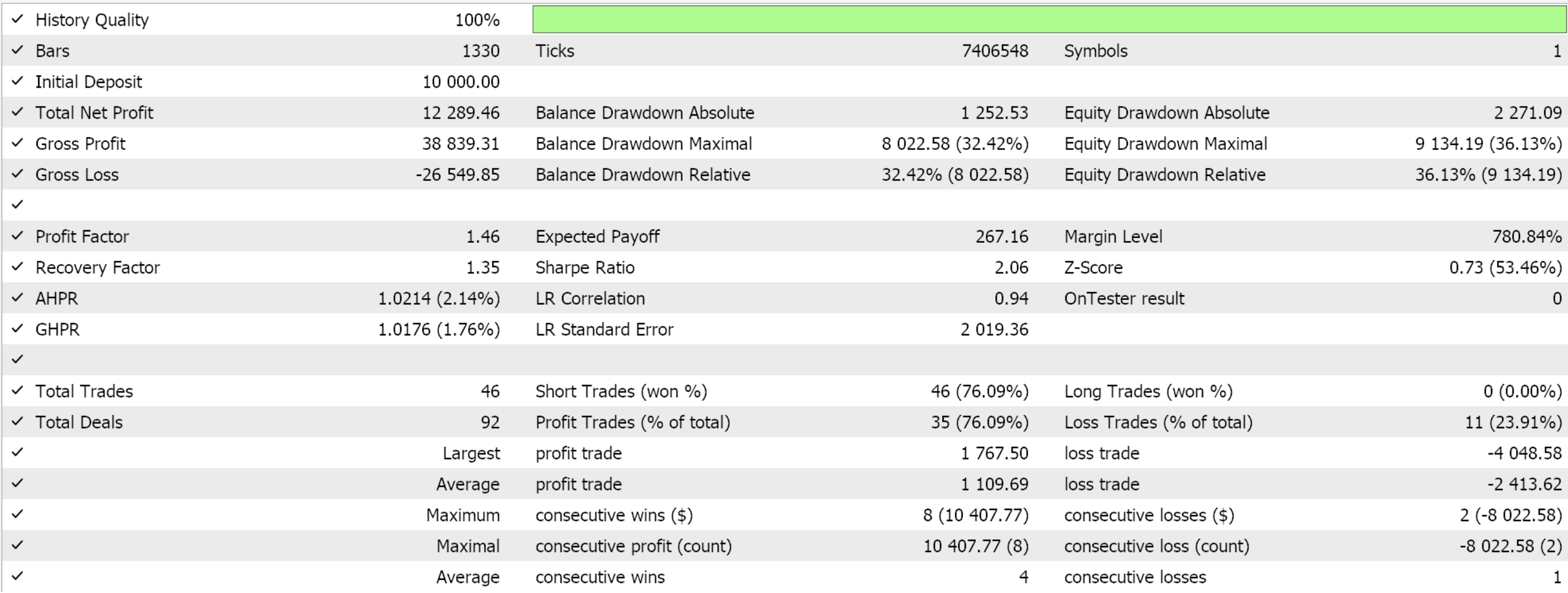
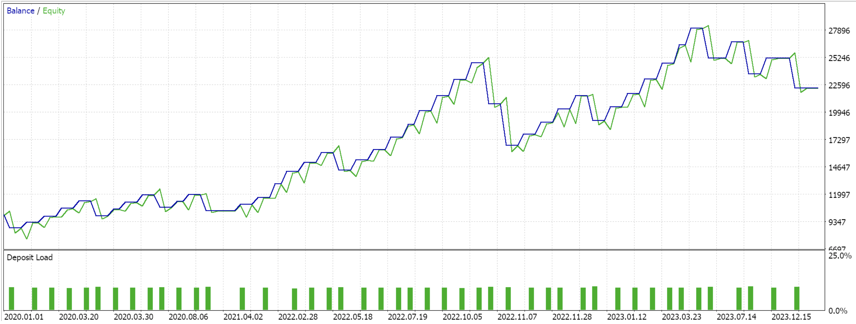
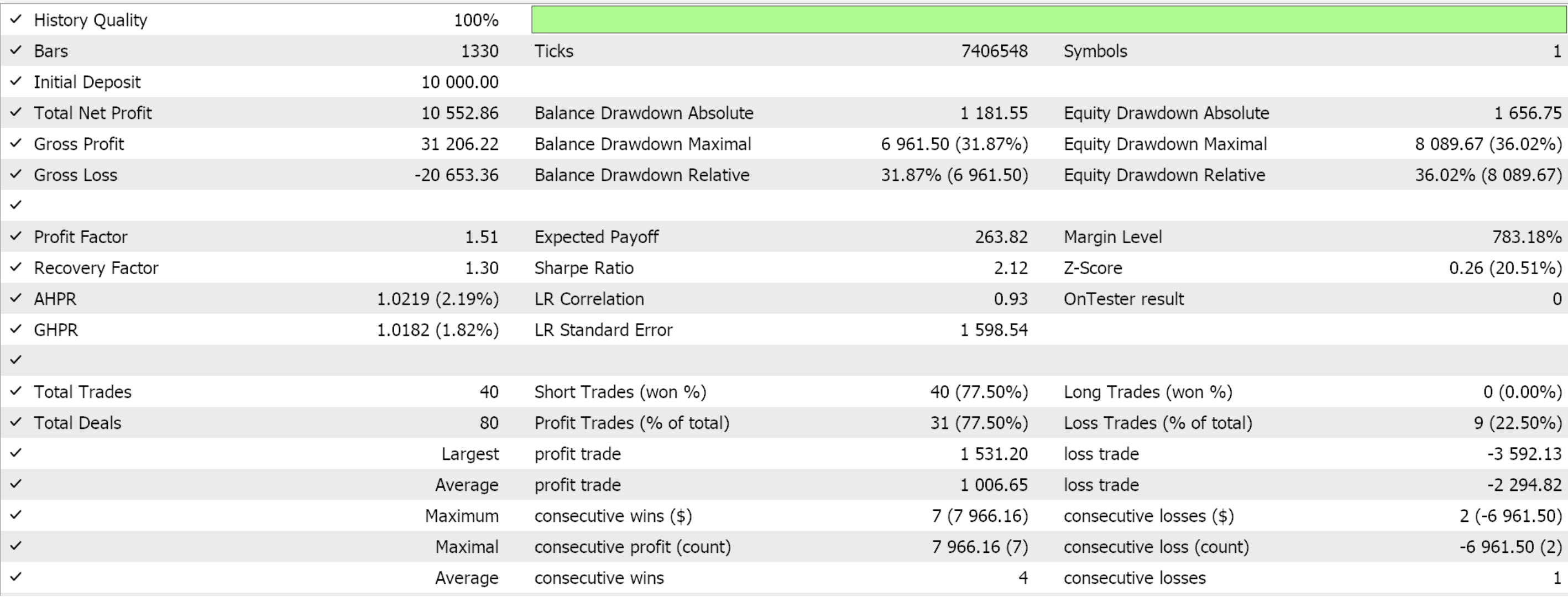
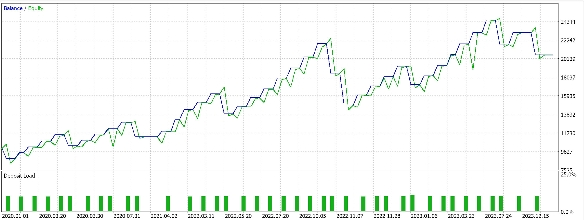
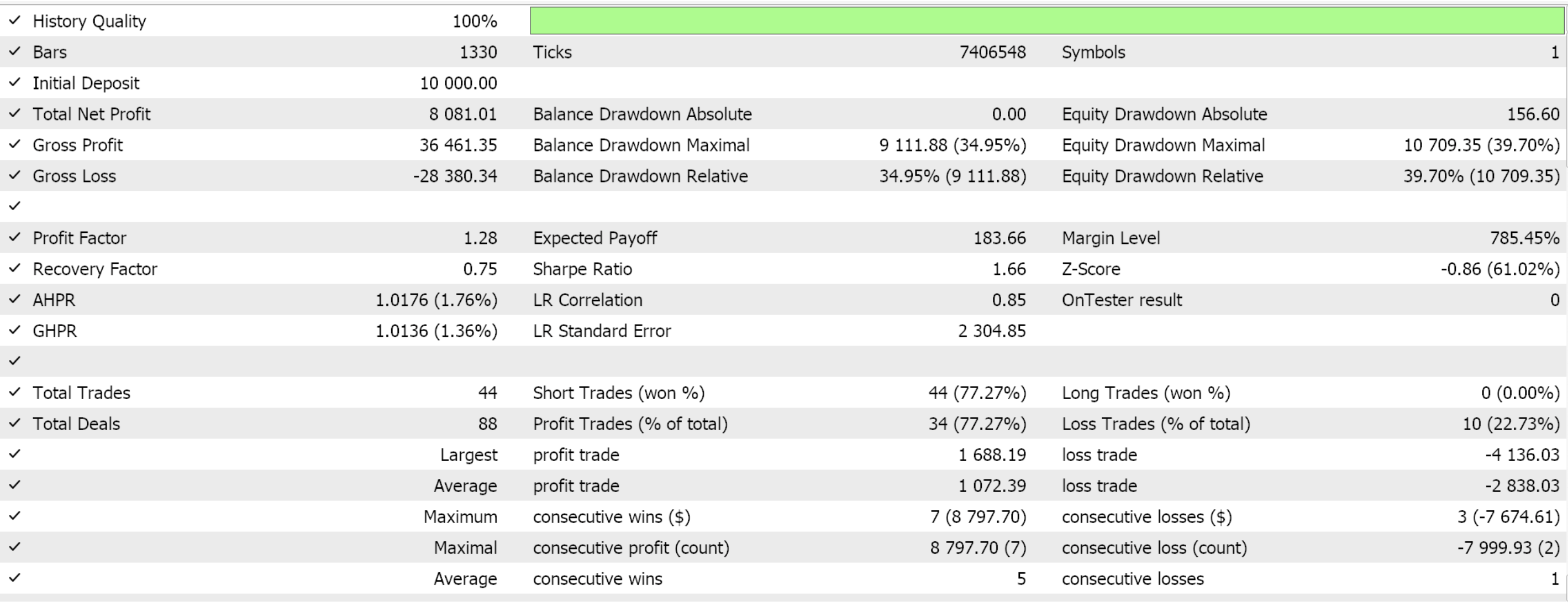
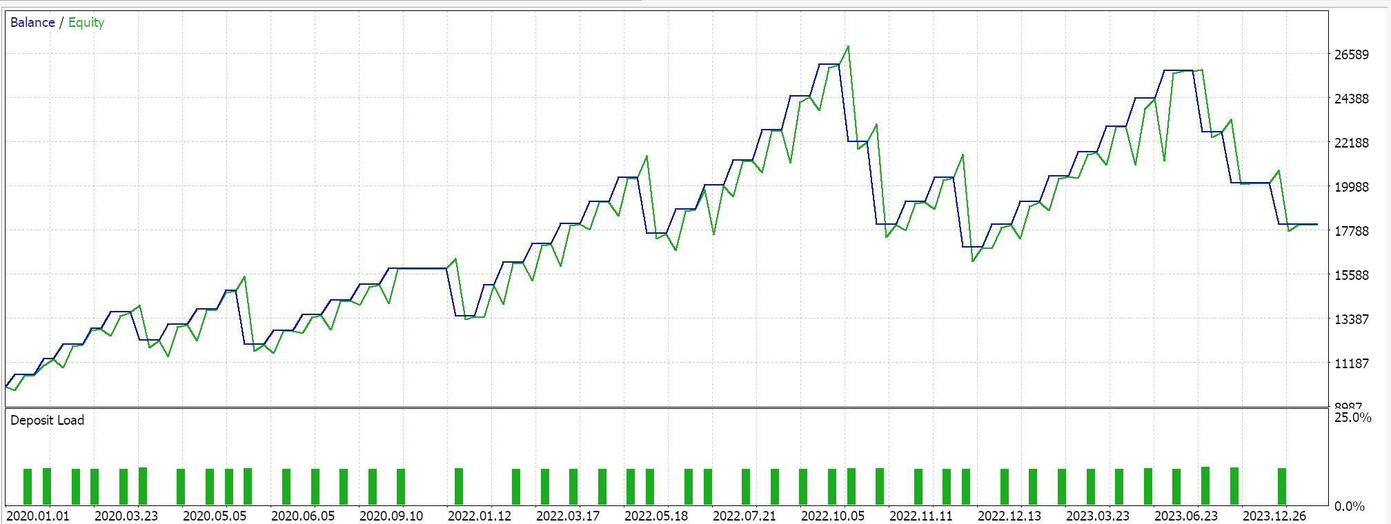
If we consider that the forward walk period is only the year 2024, then it seems only patterns 2 and 3 were able to walk. As always, many factors are at play and independent diligence is always recommended before using any code/ material shared in these articles. To assemble and use Expert Advisors such as the one used in the tests above, one needs to use files of the attached code with the MQL5 wizard. For new readers, there is guidance here and here on how to do that.

Conclusion

We have followed up our last article on how a supervised-learning model that takes as inputs patterns of the ADX and CCI can be developed into an Expert Advisor with another article. This article uses the same indicators but in reinforcement learning. RL aims to make the earlier developed Expert Advisor more robust by cautiously extending its learning window.

A sum up article that is meant to follow, for these indicator patterns, was meant to look at inference. We apply inference here as a means of summarizing and ‘archiving’ what is learnt in supervised learning and reinforcement learning. Illustrations of this approach are in this article. However, we will leave inference use to the reader as we will return to a simpler article format that will alternately feature some machine learning ideas. 

Name	Description
wz_62.mq5	Wizard Assembled Expert Advisor whose header shows files included
SignalWZ_62.mqh	Custom Signal Class File
61_2.onnx	Feature-2 ONNX Supervised Learning Model
61_3.onnx	Feature-3 ONNX Supervised Learning Model
61_4.onnx	Feature-4 ONNX Supervised Learning Model
62_policy_2.onnx	Feature-2 Reinf. Learning Actor
62_policy_3.onnx	Feature-3 Reinf. Learning Actor
62_policy_4.onnx	Feature-4 Reinf. Learning Actor
62_value_2.onnx	Feature-2 Reinf. Learning Critic
62_value_3.onnx	Feature-3 Reinf. Learning Critic
62_value_4.onnx	Feature-4 Reinf. Learning Critic