Population optimization algorithms: Simulated Annealing (SA) algorithm. Part I

Contents

1. Introduction
2. Algorithm
3. Test results

1. Introduction

The Simulated Annealing algorithm was developed by Scott Kirkpatrick, George Gelatt and Mario Vecchi in 1983. When studying the properties of liquids and solids at high temperatures, it was found that the metal transforms into a liquid state and the particles are distributed randomly, while the state with minimum energy is achieved under the condition of a sufficiently high initial temperature and a sufficiently long cooling time. If this condition is not fulfilled, then the material will find itself in a metastable state with non-minimum energy - this is called hardening, which consists of sharp cooling of the material. In this case, the atomic structure has no symmetry (anisotropic state, or uneven properties of the material inside the crystal lattice).

During the slow annealing process, the material also turns into a solid state, but with organized atoms and with symmetry, so it was proposed to use this process to develop an optimization algorithm that could find a global optimum in complex problems. The algorithm has also been proposed as a method for solving combinatorial optimization problems.

Thus, the main idea of the algorithm is based on a mathematical analogue of the metal annealing process. During the annealing process, in order to evenly distribute its internal energy, the metal is heated to a high temperature and then slowly cooled, allowing the metal molecules to move and order into more stable states, while internal stresses in the metal are relieved and intercrystalline defects are removed. The term "annealing" is also associated with thermodynamic free energy, which is an attribute of the material and depends on its state.

The simulated annealing optimization algorithm uses a similar process. The algorithm applies operations similar to heating and cooling the material. The algorithm begins its work with an initial solution, which can be random or obtained from previous iterations. Then it applies operations to change the state of the solution, which can be random or controlled, to obtain a new state, even if it is worse than the current one. The probability of making a worse decision is determined by a "cooling" function, which reduces the probability of making a worse decision over time, allowing the algorithm to temporarily "jump out" of local optima and look for better solutions elsewhere in the search space.

The simulated annealing algorithm is based on three main concepts:

• Application of randomness: The algorithm uses random operations to change the state of the solution and select the next state. This allows exploring different regions of the search space and avoid getting stuck in local optima.

• Accepting worse decisions: SA is one of the very few algorithms that prefers worse decisions with some probability to better decisions.

• Gradually reducing the likelihood of making worse decisions: The algorithm uses a "cooling" process that reduces the likelihood of making worse decisions over time. This allows us to first explore the search space more broadly and then focus on improving the solution, balancing exploration and exploitation of the search space.

The simulated annealing optimization algorithm is one of the methods used in metaheuristics, which describes a class of algorithms for solving complex optimization problems. They are based on heuristic methods that allow searching for approximate solutions in the search space without requiring a complete search of all possible options. Randomness is one of the key elements of metaheuristics that allows them to discover new and promising solution regions. The algorithm belongs to a group of algorithms called "stochastic optimization methods".

The SA algorithm has its disadvantages, which we will discuss below. Other algorithms based on SA have been developed, such as Adaptive Simulated Annealing (ASA) and Quantum Normalization (QN) also known as Quantum Annealing (QA).

2. Algorithm

The basic version of the simulated annealing algorithm proposed by the authors is extremely simple, but it is not easy to imagine how the algorithm works without visually displaying graphs of the temperature change process and a graph of the probability of making worst decisions.

Let's figure it out step by step. The algorithm starts working with a certain initial high temperature (external parameter), which corresponds to the heating of the material in metallurgy. High temperature means high energy of molecules moving from different energy states (either lower or higher). Similar to this process of high-energy motion in metal, the system can make worse decisions with some probability.

If we imagine the movement of a skier from the top of a mountain, then when he finds himself in some local lowland, the skier may decide that he has reached the foot of the mountain. In order to make sure that the decision is correct, we need to slightly worsen our position and rise to some height to rush down with even greater speed. This is the point of making worse decisions with some probability. In order to jump out of the local "trap", a quantum annealing algorithm was developed that simulates the quantum effects of being in two places at the same time, where it is supposed to jump over "walls" using tunneling, but trying to get rid of some disadvantages, quantum annealing received others, in particular the problem of choosing the strength of a quantum transition.

Several simple equations are used to describe simulated annealing. Energy calculation equation:

E = f (x)

In other words, E represents the value of the fitness function for the current state of the agent.

Energy change calculation equation:

ΔE = E_new - E_old

where:

• ΔE - change in energy during the transition from the current state to a new one (the difference in the values of the fitness function at two successive iterations)
  
• E_new - energy value for the new state
• E_old - energy value for the previous state

Equation for calculating the probability of making a worse decision:

P = exp (-ΔE / T)

where:

• P - probability of making a worse decision
• T - current temperature

From the graph below, which shows the P probability dependence, it is clear that the higher ΔE corresponds to a lower probability. This means that as temperature decreases, the probability of high-energy downward transitions decreases faster than transitions with smaller energy differences. In other words, the algorithm takes less and less risk in trying to get out of the "trap" preferring only to improve the solution. The probability plot is shown in Figure 1, using a linear decrease in temperature for clarity, although the algorithm uses a non-linear change in temperature.

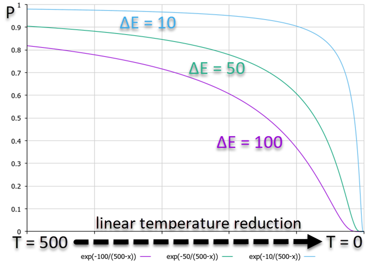
Figure 1. Graph of decision-making probabilities depending on energy changes for the worse with a linear decrease in temperature

Temperature update equation:

Tnew = α * Tprev

where:

• α - cooling ratio. α is usually in the range from 0.8 to 0.99
• Tnew - new temperature
• Tprev - previous temperature
  

The graph of temperature change at each iteration with α = 0.99, 0.8, 0.5 and 0.1 at the starting temperature T = 500 is shown in Figure 2. The temperature gradually decreases, which corresponds to the cooling of the material. Reducing the temperature at each iteration leads to a decrease in the probability of making worse decisions, which corresponds to a decrease in the ability of molecules to change their energy state as the temperature decreases.

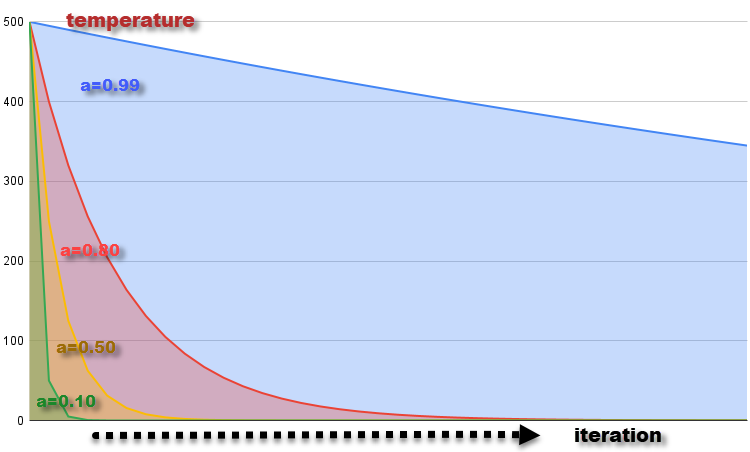
Figure 2. Temperature change graph with α = 0.99, 0.8, 0.5 and 0.1

Equation for generating a new system state:

x_new = GenerateNeighbor (x)

where:

• x_new - a new state generated based on the current x state
  
• GenerateNeighbor (x) - the function that generates a new state by introducing random changes with a uniform distribution to the current state
  

Now that we know all the theoretical foundations of the simulated annealing algorithm, it will not be difficult for us to write SA code. We can represent the movement of molecules that change their energy state in the form of a structure (S_Agent), which contains information about the agent in the optimization problem. Fields and structure methods:

• Init (int coords) - method initializes the agent and allocates memory for the "c" and "cPrev" arrays of "coords" size. It also sets the initial values of "f" and "fPrev" to "-DBL_MAX" (negative infinity)
• c [] - "c" array represents the agent's coordinates in the optimization space
  
• cPrev [] - "cPrev" array represents the agent's previous coordinates
  
• f - the fitness function value for the agent's current coordinates
  
• fPrev - the previous value of the agent's fitness function
  

//————————————————————————————————————————
struct S_Agent
{
  void Init (int coords)
  {
    ArrayResize (c,     coords);
    ArrayResize (cPrev, coords);
    f     = -DBL_MAX;
    fPrev = -DBL_MAX;
  }

  double c     []; //coordinates
  double cPrev []; //previous coordinates
  double f;        //fitness
  double fPrev;    //previous fitness
};
//————————————————————————————————————————

Let's describe the SA algorithm class and call it C_AO_SA. It will turn out to be very simple, since it does not contain anything unusual we have not used before, except for specific thermal variables and constants.

Class fields and methods:

• cB [] - array of the best coordinates found by the optimization algorithm at the time of the current iteration
  
• fB - fitness function value for the best coordinates
  
• a [] - the array represents agents. It is used to store information about each agent in an optimization problem. Each element of the array is an instance of the S_Agent structure
• rangeMax [] - array of maximum search range values for each coordinate used to determine the upper search border for each agent coordinate
• rangeMin [] - array of minimum search range values for each coordinate used to determine the lower search border for each agent coordinate
• rangeStep [] - the array represents search steps for each coordinate
• Init (const int coordsP, const int popSizeP, const double tP, const double aP, const double dP) - the method initializes the optimization algorithm, accepts parameters: number of coordinates "coordsP", population size "popSizeP", initial temperature "tP", temperature reduction ratio "aP" and diffusion coefficient "dP". The method initializes the class and agent fields
• Moving () - the method moves the agents during optimization and uses the algorithm to determine agents' new coordinates
• Revision () - the method performs a revision and update of the best coordinates and fitness function based on the current values of the agents
• SeInDiSp (double In, double InMin, double InMax, double Step) - the private method used to normalize the value of "In" in the range from "InMin" to "InMax" with a step of "Step"
• RNDfromCI (double min, double max) - private method used to generate a random number in a given range from "min" to "max"

It should be noted that the dP diffusion ratio is not present in the original SA version. The authors’ idea was to generate a new state of the system and, accordingly, a new coordinate of agents over the entire range from "min" to "max" for each coordinate. This would correspond to the chaotic movement of molecules in the entire "volume" of the metal subjected to annealing. My experiments have shown that the results improve if the range of molecular vibrations is limited to only a certain interval expressed in parts of the entire permissible interval. This is the exact objective of the diffusion ratio parameter - to limit the area of possible mixing of molecules.

To obtain results equivalent to the original SA, simply set the parameter to 1 (default 0.2).

//————————————————————————————————————————
class C_AO_SA
{
  //----------------------------------------------------------------------------
  public: double  cB [];  //best coordinates
  public: double  fB;     //FF of the best coordinates
  public: S_Agent a  [];  //agent

  public: double rangeMax  []; //maximum search range
  public: double rangeMin  []; //manimum search range
  public: double rangeStep []; //step search

  public: void Init (const int    coordsP,      //coordinates number
                     const int    popSizeP,     //population size
                     const double tP,           //temperature
                     const double aP,           //temperature reduction coefficient
                     const double dP);          //diffusion coefficient


  public: void Moving   ();
  public: void Revision ();

  //----------------------------------------------------------------------------
  private: int    coords;       //coordinates number
  private: int    popSize;      //population size

  private: double T;
  private: double α;
  private: double d;

  private: bool   revision;

  private: double SeInDiSp  (double In, double InMin, double InMax, double Step);
  private: double RNDfromCI (double min, double max);
};
//————————————————————————————————————————

The Init function will serve as the initialization method, which initializes all fields of the class and distributes the sizes of the necessary arrays for the optimization algorithm to work.

//————————————————————————————————————————
void C_AO_SA::Init (const int    coordsP,      //coordinates number
                    const int    popSizeP,     //population size
                    const double tP,           //temperature
                    const double aP,           //temperature reduction coefficient
                    const double dP)           //diffusion coefficient
{
  MathSrand ((int)GetMicrosecondCount ()); // reset of the generator
  fB       = -DBL_MAX;
  revision = false;

  coords     = coordsP;
  popSize    = popSizeP;
  T          = tP;
  α          = aP;
  d          = dP;

  ArrayResize (a, popSize);
  for (int i = 0; i < popSize; i++) a [i].Init (coords);

  ArrayResize (rangeMax,  coords);
  ArrayResize (rangeMin,  coords);
  ArrayResize (rangeStep, coords);
  ArrayResize (cB,        coords);
}
//————————————————————————————————————————

Write the Moving method to move agents in the search space.
At the first iteration, when the algorithm has just been launched, the variable - "revision" flag is equal to "false". It is necessary to initialize the population agents with initial values lying in the range of [min;max] coordinates with a uniform distribution. We normalize the obtained values of the agents’ coordinates with the SeInDiS function in order to maintain the required movement step. Next, the "revision" flag is set to "true" to indicate that the simulated annealing algorithm operators will need to be applied in the next iteration.

If this were the original SA, then we would do what we did in the first iteration, i.e. would continue to generate random numbers in a given range with a uniform distribution in the second and subsequent iterations. In our slightly corrected version, we will do the same, but with adjustment of the range of values, thereby limiting the area of diffusion interaction of molecules in the metal, while the movement is carried out from the place where the molecule was at the previous iteration. We normalize the obtained values of the agents’ coordinates with the SeInDiS function in order to maintain the required movement step.

//————————————————————————————————————————
void C_AO_SA::Moving ()
{
  //----------------------------------------------------------------------------
  if (!revision)
  {
    for (int i = 0; i < popSize; i++)
    {
      for (int c = 0; c < coords; c++)
      {
        a [i].c [c] = RNDfromCI (rangeMin [c], rangeMax [c]);
        a [i].c [c] = SeInDiSp (a [i].c [c], rangeMin [c], rangeMax [c], rangeStep [c]);
      }
    }

    revision = true;
    return;
  }

  //----------------------------------------------------------------------------
  double rnd = 0.0;

  for (int i = 0; i < popSize; i++)
  {
    for (int c = 0; c < coords; c++)
    {
      rnd = RNDfromCI (-0.1, 0.1);
      a [i].c [c] = a [i].cPrev [c] + rnd * (rangeMax [c] - rangeMin [c]) * d;
      a [i].c [c] = SeInDiSp (a [i].c [c], rangeMin [c], rangeMax [c], rangeStep [c]);
    }
  }
}
//————————————————————————————————————————

While in the "Moving" method we generated new states of the system, i.e. moved molecules in the molten metal, then in the "Revision" method we will calculate the "heat balance" and the probability of the molecules transitioning to a new state.

At the beginning of the method, we will check the values of all fitness functions of the agents. If we find values better than the global one, then we will update it.

Next, in the “for” loop, perform the following actions for each agent in the population:

• the value "ΔE" is calculated as the absolute value of the difference between "a[i].f" and "a[i].fPrev", i.e. the difference between the values of the fitness function at the current and previous iteration

If the value of "a[i].f" is greater than the value of "a[i].fPrev" (i.e., the current fitness is better than the previous one), then the following block of code is executed:

• the value "a[i].fPrev" is replaced with "a[i].f"
• the values of the "a[i].cPrev" array are copied from the "a[i].c" array

Otherwise, the following block of code is executed (the current value of the fitness function is worse than the previous one):

• the probability value "P" is calculated as the exponent of the negative ratio of "ΔE" to "T"
• generate a random number from the range [0.0;1.0] for "rnd" modeling the probability of transition to a new state that is worse than the previous one

If the value of "rnd" is less than the value of "P" (i.e., the probability is fulfilled), then:

• the value "a[i].fPrev" is replaced with "a[i].f"
• the values of the "a[i].cPrev" array are copied from the "a[i].c" array

The temperature value "T" is multiplied by the "α" thermal ratio, which gives a decrease in temperature with each new iteration.

//————————————————————————————————————————
void C_AO_SA::Revision ()
{
  //----------------------------------------------------------------------------
  int ind = -1;

  for (int i = 0; i < popSize; i++)
  {
    if (a [i].f > fB) ind = i;
  }

  if (ind != -1)
  {
    fB = a [ind].f;
    ArrayCopy (cB, a [ind].c, 0, 0, WHOLE_ARRAY);
  }

  //----------------------------------------------------------------------------
  double rnd  = 0.0;
  double ΔE;
  double P;

  for (int i = 0; i < popSize; i++)
  {
    ΔE = fabs (a [i].f - a [i].fPrev);

    if (a [i].f > a [i].fPrev)
    {
      a [i].fPrev = a [i].f;
      ArrayCopy (a [i].cPrev, a [i].c, 0, 0, WHOLE_ARRAY);
    }
    else
    {
      P = exp (-ΔE / T);
      rnd = RNDfromCI (0, 1.0);

      if (rnd < P)
      {
        a [i].fPrev = a [i].f;
        ArrayCopy (a [i].cPrev, a [i].c, 0, 0, WHOLE_ARRAY);
      }

    }
  }

  T = α * T;
}
//————————————————————————————————————————

3. Test results

Test stand results of the original algorithm with the generation of random numbers in the entire permissible range of values:

C_AO_SA:50:1000.0:0.1:0.2
=============================
5 Rastrigin's; Func runs 10000 result: 61.3646399742684
Score: 0.76034
25 Rastrigin's; Func runs 10000 result: 47.454223750487884
Score: 0.58798
500 Rastrigin's; Func runs 10000 result: 39.06494648961887
Score: 0.48404
=============================
5 Forest's; Func runs 10000 result: 0.4708272303190655
Score: 0.26632
25 Forest's; Func runs 10000 result: 0.17553657864203864
Score: 0.09929
500 Forest's; Func runs 10000 result: 0.0538869772164491
Score: 0.03048
=============================
5 Megacity's; Func runs 10000 result: 2.6
Score: 0.21667
25 Megacity's; Func runs 10000 result: 1.0
Score: 0.08333
500 Megacity's; Func runs 10000 result: 0.3044
Score: 0.02537
=============================
All score: 2.55383

Test stand results of the algorithm with the addition of the diffusion ratio:

C_AO_SA:50:1000.0:0.1:0.2
=============================
5 Rastrigin's; Func runs 10000 result: 65.78409729002105
Score: 0.81510
25 Rastrigin's; Func runs 10000 result: 52.25447043222567
Score: 0.64746
500 Rastrigin's; Func runs 10000 result: 40.40159931988021
Score: 0.50060
=============================
5 Forest's; Func runs 10000 result: 0.5814827554067439
Score: 0.32892
25 Forest's; Func runs 10000 result: 0.23156336186841173
Score: 0.13098
500 Forest's; Func runs 10000 result: 0.06760002887601002
Score: 0.03824
=============================
5 Megacity's; Func runs 10000 result: 2.92
Score: 0.24333
25 Megacity's; Func runs 10000 result: 1.256
Score: 0.10467
500 Megacity's; Func runs 10000 result: 0.33840000000000003
Score: 0.02820
=============================
All score: 2.83750

We can see that the algorithm's performance has noticeably improved by applying the diffusion ratio. The original algorithm required improvements to be included in our table. It is unexpected for such a well-known and popular optimization method to have such weak results, especially since it is applied in training neural networks.

SA visualization did not reveal any noticeable distinctive features in the behavior of agents in the search space. The points behave chaotically without forming structures similar to thermal Brownian motion. Besides, the algorithm gets stuck in local extrema and convergence leaves much to be desired, although there is no shortage of population diversity, i.e. the population is not depleted at the end of the iterations.

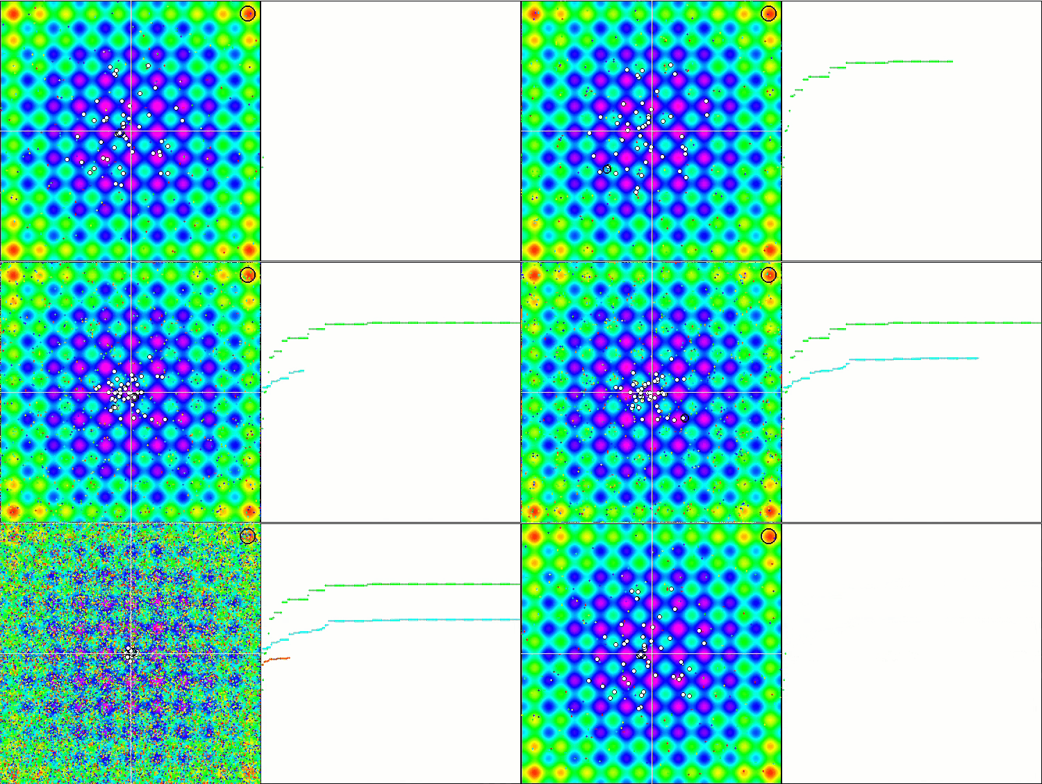
  SA on the Rastrigin test function

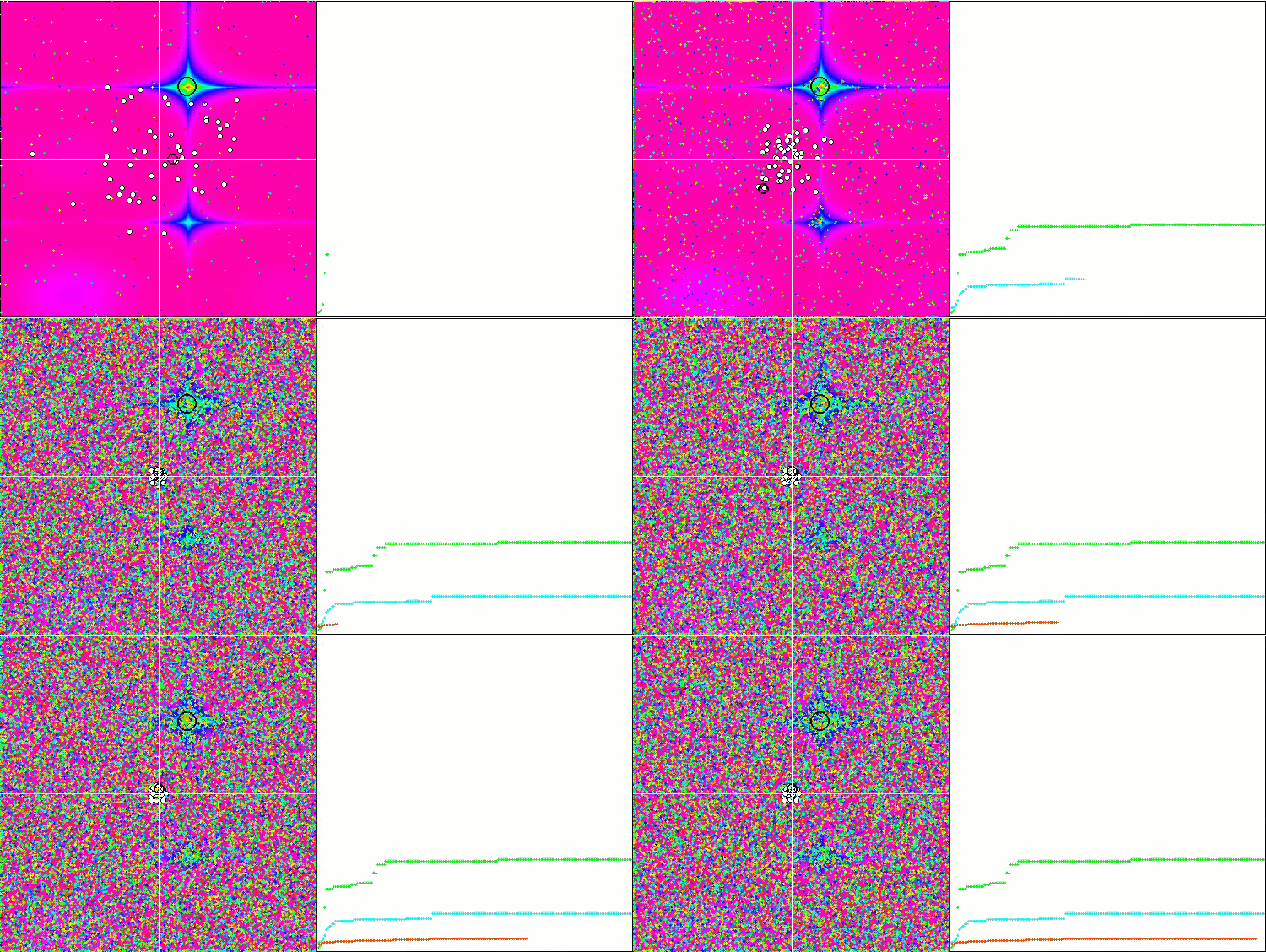
  SA on the Forest test function

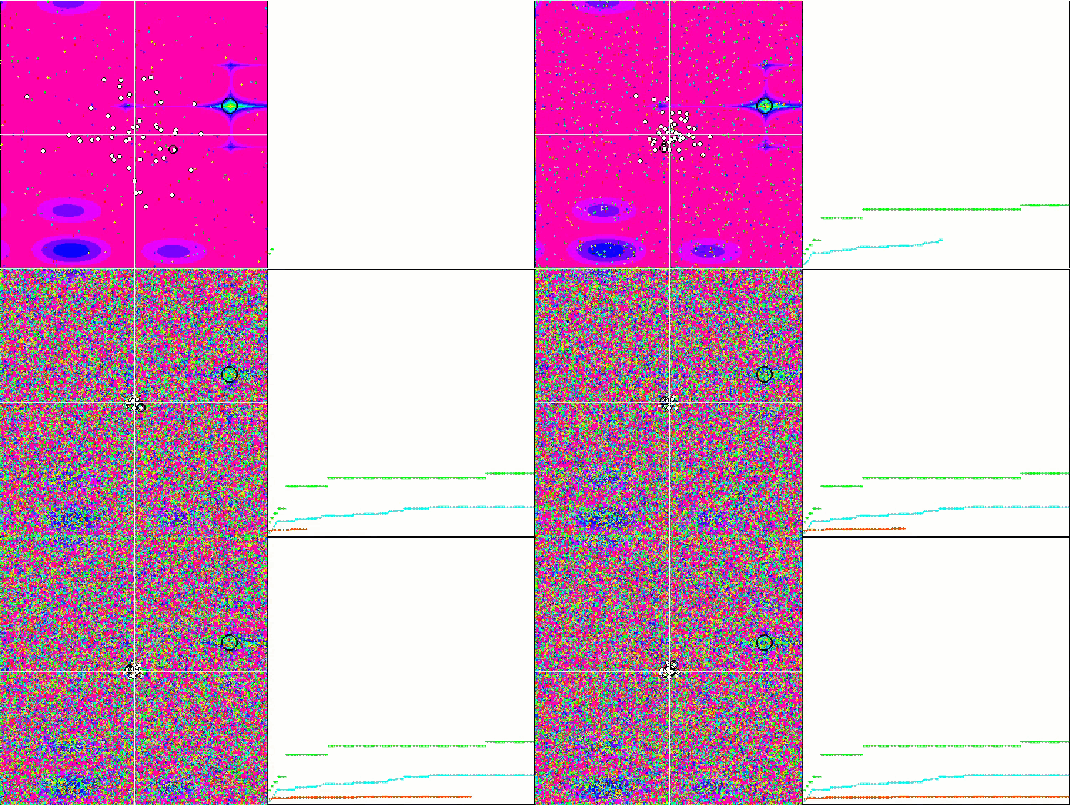
   SA on the Megacity test function

The simulated annealing algorithm ranked at the bottom of the table. The comparison table shows that the algorithm does not have any distinctive features in individual tests. All results are below average. There are algorithms in the table, such as CSS, that show excellent results in some tests, although they are at the bottom of the table. Unfortunately, the SA algorithm is not one of them.

#	AO	Description	Rastrigin			Rastrigin final	Forest			Forest final	Megacity (discrete)			Megacity final	Final result
			10 p (5 F)	50 p (25 F)	1000 p (500 F)		10 p (5 F)	50 p (25 F)	1000 p (500 F)		10 p (5 F)	50 p (25 F)	1000 p (500 F)
1	SDSm	stochastic diffusion search M	0.99809	1.00000	0.69149	2.68958	0.99265	1.00000	1.00000	2.99265	1.00000	1.00000	1.00000	3.00000	100.000
2	SSG	saplings sowing and growing	1.00000	0.92761	0.51630	2.44391	0.72120	0.65201	0.83760	2.21081	0.54782	0.61841	0.99522	2.16146	77.683
3	DE	differential evolution	0.98295	0.89236	0.51375	2.38906	1.00000	0.84602	0.65510	2.50112	0.90000	0.52237	0.12031	1.54268	73.099
4	HS	harmony search	0.99676	0.88385	0.44686	2.32747	0.99148	0.68242	0.37529	2.04919	0.71739	0.71842	0.41338	1.84919	70.623
5	IWO	invasive weed optimization	0.95828	0.62227	0.27647	1.85703	0.70170	0.31972	0.26613	1.28755	0.57391	0.30527	0.33130	1.21048	48.250
6	ACOm	ant colony optimization M	0.34611	0.16683	0.15808	0.67103	0.86147	0.68980	0.64798	2.19925	0.71739	0.63947	0.05579	1.41265	47.387
7	MEC	mind evolutionary computation	0.99270	0.47345	0.21148	1.67763	0.60244	0.28046	0.21324	1.09615	0.66957	0.30000	0.26045	1.23002	44.049
8	SDOm	spiral dynamics optimization M	0.69840	0.52988	0.33168	1.55996	0.59818	0.38766	0.37600	1.36183	0.35653	0.15262	0.25842	0.76758	40.289
9	NMm	Nelder-Mead method M	0.88433	0.48306	0.45945	1.82685	0.46155	0.24379	0.21903	0.92437	0.46088	0.25658	0.16810	0.88555	39.660
10	COAm	cuckoo optimization algorithm M	0.92400	0.43407	0.24120	1.59927	0.57881	0.23477	0.13842	0.95200	0.52174	0.24079	0.17001	0.93254	37.830
11	FAm	firefly algorithm M	0.59825	0.31520	0.15893	1.07239	0.50637	0.29178	0.41704	1.21519	0.24783	0.20526	0.35090	0.80398	33.139
12	ABC	artificial bee colony	0.78170	0.30347	0.19313	1.27829	0.53379	0.14799	0.11177	0.79355	0.40435	0.19474	0.13859	0.73768	29.766
13	BA	bat algorithm	0.40526	0.59145	0.78330	1.78002	0.20664	0.12056	0.21769	0.54488	0.21305	0.07632	0.17288	0.46225	29.499
14	CSS	charged system search	0.56605	0.68683	1.00000	2.25289	0.13961	0.01853	0.13638	0.29452	0.07392	0.00000	0.03465	0.10856	27.930
15	GSA	gravitational search algorithm	0.70167	0.41944	0.00000	1.12111	0.31390	0.25120	0.27812	0.84322	0.42609	0.25525	0.00000	0.68134	27.807
16	BFO	bacterial foraging optimization	0.67203	0.28721	0.10957	1.06881	0.39364	0.18364	0.17298	0.75026	0.37392	0.24211	0.18841	0.80444	27.542
17	EM	electroMagnetism-like algorithm	0.12235	0.42928	0.92752	1.47915	0.00000	0.02413	0.29215	0.31628	0.00000	0.00527	0.10872	0.11399	19.002
18	SFL	shuffled frog-leaping	0.40072	0.22021	0.24624	0.86717	0.19981	0.02861	0.02221	0.25063	0.19565	0.04474	0.06607	0.30646	13.200
19	SA	simulated annealing	0.36938	0.21640	0.10018	0.68595	0.20341	0.07832	0.09372	0.37545	0.16956	0.08422	0.10394	0.35772	13.138
20	MA	monkey algorithm	0.33192	0.31029	0.13582	0.77804	0.09927	0.05443	0.07482	0.22852	0.15652	0.03553	0.10669	0.29874	11.777
21	FSS	fish school search	0.46812	0.23502	0.10483	0.80798	0.12730	0.03458	0.05458	0.21647	0.12175	0.03947	0.08244	0.24366	11.332
22	IWDm	intelligent water drops M	0.26459	0.13013	0.07500	0.46972	0.28358	0.05445	0.05112	0.38916	0.22609	0.05659	0.05054	0.33322	10.423
23	PSO	particle swarm optimisation	0.20449	0.07607	0.06641	0.34696	0.18734	0.07233	0.18207	0.44175	0.16956	0.04737	0.01947	0.23641	8.426
24	RND	random	0.16826	0.09038	0.07438	0.33302	0.13381	0.03318	0.03949	0.20648	0.12175	0.03290	0.04898	0.20363	5.054
25	GWO	grey wolf optimizer	0.00000	0.00000	0.02093	0.02093	0.06514	0.00000	0.00000	0.06514	0.23478	0.05789	0.02545	0.31812	1.000

Summary

The simulated annealing algorithm has several weaknesses that may limit its effectiveness in solving some optimization problems. Some of these weaknesses include:

• Dependency on initial solution: Like many other optimization methods, the simulated annealing algorithm can depend on an initial solution, which is chosen at random. If the initial solution is bad, then the algorithm may get stuck in a local optimum and fail to find a global one.
  
  It is important to note that the algorithm requires tuning parameters such as the initial "temperature" and the temperature change step, which affect the likelihood of making a worse decision. These parameters affect the performance and quality of solutions, so parameter selection and tuning are important aspects when applying a simulated annealing algorithm to a specific optimization problem. Setting these parameters can be challenging. Incorrect setting can lead to poor results. The default settings were chosen to obtain the best results in the test feature set.
  
  
• Another weakness of the simulated annealing algorithm is the possibility of getting stuck at local extremes. This occurs when the algorithm finds an optimal solution that is a local extremum but is not a global extremum. In this case, the algorithm is not able to advance further and stops at the local optimum. This is very clearly visible in the visualization above.
  
  
• Slow convergence rate: SA can be slow in converging to an optimal solution, especially for complex optimization problems. This is because the algorithm uses randomness and may make worse decisions, which can slow down the optimization process.
  
  
• Need for a large number of iterations: To achieve an optimal solution, the simulated annealing algorithm may require a large number of iterations. This can be a problem for tasks where execution time is a critical factor.
  
  
• Low efficiency in solving problems with a large number of variables: SA may be ineffective when solving problems with a large number of variables because the search space may be too large. In this case, other optimization methods, such as genetic algorithms or gradient-based optimization methods, may be more effective. The algorithm copes well with a small number of variables (1-2), as does any algorithm, even a simple random RND.

There are several improvements that can be applied to the simulated annealing algorithm to improve its performance and efficiency:

1. Modification of the cooling function: Cooling function is an important parameter of the algorithm that regulates the cooling speed and temperature of the system.

2. Using more efficient methods for selecting the next state: SA uses random selection of the next state. However, there are more efficient methods for selecting the next state, such as mutation and crossover methods.

3. Using adaptive parameters: Algorithm parameters, such as initial temperature and cooling ratio, can be adaptively adjusted depending on the characteristics of the optimization problem.

4. Using a combination of algorithms: SA can be combined with other optimization algorithms, such as genetic algorithms or gradient descent methods, to improve optimization performance and efficiency.

The use of different distributions of a random variable when generating a new state of the system, instead of a uniform one, did not help improve the results. However, there is a way to radically transform this very well-known and popular algorithm to such an extent that it is able to compete with the leaders of the table. How is this possible? - I will share this method in the second part of the article and talk about all the stages of modification done. But, as we know, there is no universal way to improve any optimization algorithm and it depends solely on the search strategy in the algorithm itself. Therefore, the improvement will only concern the good old (but practically useless) simulated annealing algorithm.

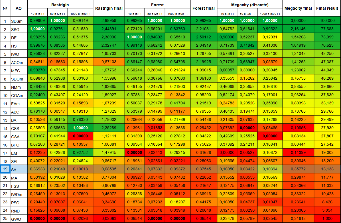
Figure 3. Color gradation of algorithms according to relevant tests

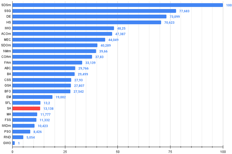
Figure 4. The histogram of algorithm test results (on a scale from 0 to 100, the more the better,

the archive contains the script for calculating the rating table using the method applied in the article)

SA pros and cons:

Advantages:

1. A small number of external parameters.
2. High operation speed.
3. Very simple implementation.
   

Disadvantages:

1. Unobvious settings (it is not clear how and what temperature affects).
   
2. Very poor scalability.
3. High scatter of results.
4. Tendency to get stuck in local extremes.
5. Poor convergence.

The article is accompanied by an archive with updated current versions of the algorithm codes described in previous articles. The author of the article is not responsible for the absolute accuracy in the description of canonical algorithms. Changes have been made to many of them to improve search capabilities. The conclusions and judgments presented in the articles are based on the results of the experiments.