MetaTrader 5 Machine Learning Blueprint (Part 24): Sequence Risk

Table of Contents

1. Introduction
2. Data and Trading Rule
3. Why Realized Drawdown Is a Single Draw
4. Block Length Is Not a Tuning Parameter
5. Breach Probability: What Prop-Firm Rules Actually Condition On
6. Walk-Forward Degradation as a Paired Difference
7. Running It on a Real EURUSD Strategy
8. Conclusion
9. Attached Files

Introduction

Earlier parts of this series, from the nested cross-validation of Part 16 to the feature screen of Part 23, ask whether a component of a trading system carries real information when it is evaluated honestly. This article asks a different question about a system that has already cleared that bar. Suppose the backtest is honest and reports a maximum drawdown of 14.3% on 820 trades. Is 14.3% the number to size an account against?

Not on its own. Maximum drawdown depends on which trades occurred and on the order in which they arrived, and both are one realization among many that the same strategy could have produced. Resample the trades and a different worst case appears, sometimes milder and sometimes much worse. Nothing guarantees that the realized draw is a typical one, and there is a selection reason to suspect a favorable one: backtests that suffered an unlucky path tend to be discarded before anyone sizes an account against them. The strategy below was fixed in advance rather than selected, and its realized drawdown sits above the median of the resampled distribution.

This article implements four tools in afml.backtest_statistics. First, a block bootstrap that resamples trade returns to estimate the drawdown distribution, together with a block permutation that keeps the realized trades and varies only their order, so that sequence risk can be separated from sampling variation. Second, breach_probability, which converts resampled trade paths into the fraction that breach a prop-firm loss limit over a stated horizon, on either a trailing or a static basis. Third, a calendar module that applies the same limits to floating equity on server-time days, which is how prop firms apply them. Fourth, a paired-difference statistic for walk-forward degradation that is reported alongside Pardo's Walk-Forward Efficiency ratio and remains defined when in-sample performance is small or negative.

Every empirical number below comes from one RSI(14) mean-reversion rule run against the attached EURUSD H1 bid and ask file for 2018 through 2024, with the bid-ask spread as its only transaction cost. Section 2 documents the file, its time zone and cleaning rules, and the exact entry and exit mechanics. Those numbers describe this rule on this quote history, and a different broker's history would move them. The methods themselves take a trade-return series (or, for the calendar check, bars plus a trade list) and do not depend on where it came from; the conclusion lists the two kinds of result separately. The walk-forward study in Section 7 adds a small grid search over the RSI thresholds, and the two-case table in Section 6 is a constructed illustration.

This is the second article in the four-part degradation-avoidance sequence that began with Part 23's feature screen. Part 25 asks how to tell, from a live stream of trade outcomes, when a deployed strategy has stopped working. Part 26 asks whether the search process that produced a strategy's parameters would have produced an equally good-looking result from data with no exploitable structure. Section 7 shows a small-scale symptom related to that question: thresholds chosen in-sample from a 4×4 grid deliver, out of sample, slightly less than an average grid point.

Data and Trading Rule

The quote file

The quote history is attached to this article as EURUSD_H1_time_2018-01-01-2024-12-31.parq. It was built from EURUSD tick history (every bid and ask quote) downloaded from FundedNext's MetaTrader 5 trade server with copy_ticks_range and the COPY_TICKS_ALL flag, then aggregated into hourly time bars by the bar builder of the data pipeline described in Part 7. Its properties:

Property	Value
Format	Apache Parquet, 43,103 rows, float32 prices, timezone-naive DatetimeIndex
Coverage	First bar 2018-01-02 00:00, last bar 2024-12-31 00:00
Columns	bid_open, bid_high, bid_low, bid_close and the four ask_ equivalents; open, high, low, close are bid-ask midpoints; spread is ask_close minus bid_close; tick_volume is the number of ticks in the bar
Time zone	Broker server time as delivered by the terminal: GMT+2, and GMT+3 during daylight saving
Time stamp	Bar close: the bar labeled 10:00 holds the ticks in [09:00, 10:00)
Cleaning	Bars with no ticks are dropped, so weekends and holidays are absent rather than forward-filled. No outlier filter or spread adjustment is applied. From August 2024 the provider's history includes Friday's last hour, so those weeks end with a bar labeled Saturday 00:00; earlier weeks end with the bar labeled Friday 23:00. Both are left as delivered
Spread	Median 0.9 pips, 99th percentile 4.4 pips
SHA-256	47bebd765c107d4627007ebfcb15ffdb1e3c8be9701ffc2ff46d99560a898fed

The reproduction script computes the file's checksum and records whether it matches, so a reader can tell a different copy of the data from a change in the code. Because the ticks come from the same FundedNext server whose midnight resets the daily loss limit in Section 5, the server days in the file are the days that rule uses.

The trading rule

RSI(14) is computed with Wilder smoothing, an exponential average of gains and losses with weight 1/14, on the mid close of each bar. When bar i has closed with RSI below 30, a long is opened; above 70, a short. The fill is the close quote of bar i + 1: the ask for a long, the bid for a short. The position exits at the close quote of bar i + 21, twenty bars after entry, at the bid for a long and the ask for a short. No signal is read until the bar after the exit, so positions never overlap. Exposure is one times notional, and returns compound from trade to trade.

The signal on bar i uses closes through bar i only, since RSI is a recursive average of past price changes, and the fill takes place a full bar later at a price that did not exist when the signal was formed. Filling at the close of bar i + 1 rather than at its open gives up an hour of the move, which makes the rule's results slightly conservative rather than optimistic. In the walk-forward study, thresholds are chosen from trades whose entry and exit both fall inside the in-sample period and scored on trades that lie wholly inside the following period.

import pandas as pd
from part24_reproduce import RSIReversionBacktest

bars = pd.read_parquet("EURUSD_H1_time_2018-01-01-2024-12-31.parq")
trades = RSIReversionBacktest(bars).trades()   # entry_time, exit_time, side, return
trade_returns = trades["return"].to_numpy()    # 820 per-trade returns, 1x notional

The other code blocks continue from these three variables.

Why Realized Drawdown Is a Single Draw

The tool for this is the stationary bootstrap of Politis and Romano (1994), already built for the null-generation work in Part 23 and reused here for a different purpose. There, resampling a series under a null answered whether a feature carries information. Here, resampling the realized trade sequence answers a question with no null hypothesis behind it: if future trades come from the same distribution as past ones, how bad can the worst case plausibly get?

The scope is worth stating precisely, because it is easy to overclaim. The stationary bootstrap draws blocks of consecutive trades with replacement, so each resampled path has the original length but its own mix of trades. It varies the ordering and the sample composition together, which is why resampled paths do not share the realized total return. Its drawdown tail therefore measures sequence risk and sampling variation combined, not sequence risk alone.

To separate the two, the module also provides a block permutation. The series is cut into blocks of the same geometric lengths, and the blocks are reordered without replacement. Every replicate then contains each realized trade exactly once, so the composition and the total return are fixed and only the ordering varies. The gap between the two distributions is the part of the tail that comes from the trades themselves being a sample. The core of both index generators and of the drawdown calculation:

# Condensed from afml/screening/permutation.py and afml/backtest_statistics/bootstrap.py
import numpy as np


def stationary_bootstrap_indices(n, mean_block, n_perm, rng):
    """Geometric blocks drawn with replacement, wrapped circularly."""
    positions = np.arange(n)
    out = np.empty((n_perm, n), dtype=np.int64)
    for k in range(n_perm):
        restarts = rng.random(n) < 1.0 / mean_block   # open a new block here?
        restarts[0] = True
        starts = rng.integers(0, n, size=n)           # random origin for each block
        block_start = np.maximum.accumulate(np.where(restarts, positions, 0))
        out[k] = (starts[block_start] + positions - block_start) % n
    return out


def block_permutation_indices(n, mean_block, n_perm, rng):
    """The same geometric blocks, reordered without replacement."""
    positions = np.arange(n)
    out = np.empty((n_perm, n), dtype=np.int64)
    for k in range(n_perm):
        cuts = rng.random(n) < 1.0 / mean_block
        cuts[0] = True
        block_id = np.cumsum(cuts) - 1
        rank = rng.permutation(block_id[-1] + 1)      # shuffled order of the blocks
        out[k] = positions[np.lexsort((positions, rank[block_id]))]
    return out


def max_drawdown_rows(R):
    """Maximum drawdown of each path; the starting balance is the first peak."""
    equity = np.cumprod(1.0 + R, axis=1)
    equity = np.concatenate([np.ones((R.shape[0], 1)), equity], axis=1)
    peak = np.maximum.accumulate(equity, axis=1)
    return (1.0 - equity / peak).max(axis=1)

The shipped functions add input validation and process replicates in chunks to bound memory; the arithmetic is the same. Usage, with the seeds that produced the numbers in Section 7:

from afml.backtest_statistics.bootstrap import (
    bootstrap_drawdown_distribution,
    sequence_risk_ratio,
)

kw = dict(mean_block=50, n_boot=10_000, seed=1)
dd_both = bootstrap_drawdown_distribution(trade_returns, **kw)    # order + composition
dd_order = bootstrap_drawdown_distribution(
    trade_returns, scheme="block_permutation", **kw)              # order only
ratio = sequence_risk_ratio(trade_returns, quantile=0.95, **kw)

Both schemes rest on the same assumption: future trades come from the same distribution and dependence structure as the realized ones. For seven years of EURUSD that is a strong assumption, and Section 7 tests it. Neither scheme captures regime change. That question is addressed by the combinatorial purged cross-validation work in this series, which varies the data the model sees rather than the outcomes it produced. CPCV asks whether the edge holds across data the model never trained on; the bootstrap asks, given the trade distribution the backtest produced, how unlucky a path of comparable trades can plausibly be.

Block Length Is Not a Tuning Parameter

Trade returns from overlapping or serially dependent labels are not exchangeable observations, and a resampling scheme that ignores the dependence can understate the tail it is meant to measure. The mean block length is not a knob to adjust until a result looks better. It encodes an assumption about how many consecutive trades share dependence, and it can fail in two directions.

Too short. A block length of one discards any clustering in the trade sequence, such as streaks of correlated outcomes or runs of large trades that arise when a strategy stays exposed to the same regime across several signals. The resampled paths then look more independent than the real trades are, and the drawdown tail can be understated.

Too long. The stationary bootstrap wraps the series circularly, so as the mean block approaches the length of the series, each replicate becomes a circular rotation of the realized sequence. A rotation can cut the realized worst stretch, which lowers the drawdown, or join a losing end of the series to a losing start, which raises it. The estimate then moves toward the drawdown distribution of the rotations of one path, not toward a fixed value, and the resampling no longer represents alternative histories. A block permutation with a single block returns the realized path itself. A sequence_risk_ratio near 1.0 is therefore not evidence that a strategy is immune to sequence risk until the block length has been checked.

For overlapping triple-barrier labels, suggested_block_length from Part 23 gives a starting point: five times the mean label span, with a floor of 50. The label span measures the overlap that makes consecutive returns dependent, and the multiple of five comes from the test-size calibration in Part 23. For non-overlapping trades, such as the ones in Section 7, there is no overlap to measure. The function returns its floor, and the floor is a default rather than a derived value. A result reported at that single block length inherits the arbitrariness of the default, so Section 7 reports the range of results across block lengths and treats the value at 50 as one point in it.

Dependence that does not come from overlap is not measured by the label span at all. Volatility regimes that make large trades cluster are the common case. For such series, test the trade returns and their absolute values for serial correlation directly. The Ljung-Box statistic at lag m is a joint test of the first m autocorrelations, and reporting it at twenty lags is a family of twenty tests, so the p-values need a multiple-testing adjustment across the lags reported. Section 7 applies Holm's step-down adjustment, which is valid under any dependence between the tests.

Breach Probability: What Prop-Firm Rules Actually Condition On

A prop-firm loss limit is a condition on a path, not on a distribution of returns. A strategy whose realized history never touched a 10% limit reports a breach probability of exactly zero when that probability is estimated from the realized history alone. It reports zero regardless of how close the realized path came to the line, or how easily a different sequence of comparable trades would have crossed it.

Modeling a rule correctly requires its basis, its horizon, its clock, and the equity it is checked on. FundedNext's Stellar 2-Step accounts serve as the example. The overall limit is 10% of the initial balance with the floor fixed at 90% of that balance (the allowed loss grows with profits, so the floor does not move): a static basis. The daily limit is 5% of the initial balance, measured as the day's closed results plus the floating results of open positions, and resets at 00:00 server time, which is GMT+2, or GMT+3 during daylight saving. Both limits count floating losses.

Trade-level estimate

breach_probability resamples trades and evaluates each path's compounded equity at trade exits. The drawdown_basis argument selects how the overall loss is measured: "peak" measures it from the running equity peak (a trailing limit), and "initial" measures it from the starting balance (a static floor). The horizon argument sets the number of trades per resampled path. It matters as much as the limit itself, because a longer path has more chances to breach. The same strategy can have a negligible breach probability over a few months and a large one over seven years. The check itself:

# Condensed from breach_probability(): one row per resampled path of h trades
rng = np.random.default_rng(1)
idx = stationary_bootstrap_indices(trade_returns.size, 50, 10_000, rng)
h, drawdown_basis, max_drawdown_limit = 117, "initial", 0.10

paths = trade_returns[idx][:, :h]
equity = np.concatenate([np.ones((len(paths), 1)), np.cumprod(1.0 + paths, axis=1)], axis=1)
if drawdown_basis == "peak":   # trailing: loss from the running peak
    loss = 1.0 - equity / np.maximum.accumulate(equity, axis=1)
else:                          # static: loss below the initial balance
    loss = 1.0 - equity
p_breach = (loss.max(axis=1) >= max_drawdown_limit).mean()

This estimate makes two simplifications. Equity is evaluated at trade exits only, so intra-trade excursions are invisible: for a rule checked on floating equity the estimate can understate the breach probability and cannot overstate it. An optional daily limit groups trades_per_day consecutive trades into one "day", because once the trade order has been resampled the original calendar no longer applies. That grouping matches the calendar only for a strategy that closes the stated number of trades on every day.

Calendar-day estimate on floating equity

The calendar module removes both simplifications. mark_to_market_days marks the open position to market on every bar, records the worst equity inside each bar (bid low for a long, ask high for a short), and reduces the bar path to one row per server day: equity at the previous midnight, closed balance at the start of the day, the day's floating trough, and its close. calendar_breach_probability resamples whole days in stationary-bootstrap blocks, rebuilds each path's equity from the daily ratios, and applies the rules:

# Condensed from calendar_breach_probability(): days resampled, rules on floating equity
from afml.backtest_statistics.calendar import mark_to_market_days

days = mark_to_market_days(bars, trades)   # one row per server day
rel = days[["equity_close", "equity_low", "balance_open"]].to_numpy()
rel = rel / days[["equity_open"]].to_numpy()
idx = stationary_bootstrap_indices(len(rel), 111, 2_000, np.random.default_rng(1))
g, w, b = (rel[idx][:, :260, k] for k in range(3))

e_open = np.concatenate([np.ones((len(g), 1)), np.cumprod(g, axis=1)[:, :-1]], axis=1)
low = e_open * w                                          # floating trough of each day
static_breach = low.min(axis=1) <= 1.0 - 0.10             # 10% floor below the initial balance
daily_breach = ((e_open * b - low) >= 0.05).any(axis=1)   # 5% of initial, from the midnight balance

A complete call of both estimators:

from afml.backtest_statistics.bootstrap import breach_probability
from afml.backtest_statistics.calendar import (
    calendar_breach_probability,
    realized_account_checks,
)

# Trade level: equity at exits only, consecutive trades grouped into "days"
trade_level = breach_probability(
    trade_returns, mean_block=50, max_drawdown_limit=0.10, drawdown_basis="initial",
    daily_loss_limit=0.05, trades_per_day=1, horizon=117, n_boot=100_000, seed=1)

# Calendar level: floating equity on server days, days resampled in blocks
checks = realized_account_checks(days)   # extremes of the realized path
calendar_level = calendar_breach_probability(
    days, mean_block=111, max_drawdown_limit=0.10, daily_loss_limit=0.05,
    drawdown_basis="initial", horizon=260, n_boot=100_000, seed=1)
# keys: p_drawdown_breach, p_daily_breach, p_any_breach, each with _lo/_hi bounds

Three approximations remain, and they are stated in the module rather than hidden. Bar highs and lows carry no time order, so the worst equity of a bar is treated as reachable at any point in that bar. A position open across midnight links two days, and at a block boundary the resampled path joins two days that were not adjacent. Swap and commission are not modeled beyond the spread. One limitation follows from the design and matters for the daily rule: whole days are the resampling unit, so no resampled day can lose more than the worst observed day, scaled by the equity level. For a daily limit, the realized worst day is the evidence, and a resampled breach probability of zero adds nothing beyond it.

Walk-Forward Degradation as a Paired Difference

Pardo (2008) defines Walk-Forward Efficiency as the ratio of out-of-sample to in-sample performance, with values near 1.0 read as evidence against overfitting; afml computes it as the ratio of mean scores across windows. The ratio answers a relative question, namely what fraction of in-sample performance survived out of sample. Because it is unitless, it cannot say how much score was lost. Two constructed cases with an identical ratio show the difference:

Case	Mean IS	Mean OOS	WFE ratio	Paired degradation
A	2.00	1.00	0.50	1.000
B	0.02	0.01	0.50	0.010

Case A loses a full point of score per walk-forward window. Case B loses a hundredth of a point. The ratio reports 0.50 for both, and for its own question that answer is correct: both cases kept half their in-sample score. The table does not show that the ratio is wrong. It shows that the ratio cannot distinguish the two cases, while a decision about whether a strategy is still worth trading usually needs the loss in score units. The ratio has a second limitation: a ratio of means has no simple sampling distribution, and its usual delta-method approximation breaks down as the denominator approaches zero, which is also where the ratio itself becomes unstable.

The paired difference di = ISi − OOSi is measured in the same units as the score, and its sampling distribution can be estimated by block bootstrap over windows. The default block length is 2.0 because adjacent windows overlap in data and are not independent. In the annual design of Section 7, each window's out-of-sample year is the next window's in-sample year. The core computation:

# Condensed from walkforward_degradation()
from math import comb
from part24_reproduce import annual_spans, walk_forward

wf = walk_forward(RSIReversionBacktest(bars), annual_spans())
is_arr, oos_arr = wf["is_score"].to_numpy(), wf["oos_score"].to_numpy()
n = is_arr.size

diff = is_arr - oos_arr                                    # d_i = IS_i - OOS_i
idx = stationary_bootstrap_indices(n, 2.0, 10_000, np.random.default_rng(1))
means = diff[idx].mean(axis=1)
ci_low, ci_high = np.quantile(means, [0.05, 0.95])         # 90% interval
degrades = ci_low > 0.0                                    # whole interval above zero
k = int((diff > 0).sum())                                  # windows that degraded
sign_test_p = sum(comb(n, j) for j in range(k, n + 1)) / 2 ** n

And the shipped function, which returns the same quantities with input checks:

from afml.backtest_statistics.walkforward import walkforward_degradation

result = walkforward_degradation(wf["is_score"], wf["oos_score"],
                                 mean_block=2.0, n_boot=10_000, seed=1)
result.degrades       # True only when the whole 90% interval for IS - OOS lies above zero
result.wfe_reliable   # False if any IS window is non-positive or mean IS is within 2 SE of zero
result.sign_test_p    # one-sided sign test on the number of degraded windows

The direction of the flag is deliberate. degrades is True only when the whole bootstrap interval for IS − OOS lies above zero. An interval entirely below zero (out-of-sample scores higher than in-sample ones) returns False, as does any interval that contains zero. The name describes the data rather than a cause. Selection bias, a regime change between windows, a decaying edge and noise all produce positive degradation, and separating them needs the comparison with unselected candidates shown in Section 7.

The WFE ratio is still reported, alongside a wfe_reliable flag that turns false when any in-sample window is non-positive or the mean in-sample score is within two standard errors of zero. Those are the conditions under which the ratio is unstable or mixes signs. When the flag is false, the ratio's magnitude should not be interpreted. Its sign still carries information, but it is the same information as comparing the mean out-of-sample score with the mean in-sample score.

With the handful of windows a typical walk-forward produces, the bootstrap interval is better read as a magnitude than as a threshold. A bootstrap over six values cannot be more informative than the six values themselves, so the function also reports how many windows degraded and a one-sided sign test on that count.

Running It on a Real EURUSD Strategy

Every number in this section depends on the attached quote file and the rule in Section 2. Running part24_reproduce.py on the same file reproduces them exactly, and two runs produce identical output. A different broker's quote history, a different spread model or a different fill convention will move them.

Over 2018 through 2024 the rule produces 820 non-overlapping trades, a 51.1% win rate, and a realized maximum drawdown of 14.3%. Total compounded return across seven years is 2.8%. That is unremarkable by design: the rule was fixed in advance rather than searched for, and the point of this section is the risk statistics around that number, not the number itself.

Drawdown distribution

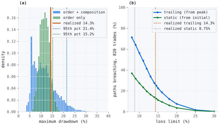
Figure 1. 2-panel illustration of drawdown resampling on 820 real EURUSD trades

• Panel (a): the distribution of maximum drawdown across 10,000 resampled paths of 820 trades at a mean block length of 50, with order and composition varied (blue) and with order alone varied (green). The blue median is 10.9%, and the realized 14.3% sits at the 74th percentile. On the green distribution the realized path sits at the 89th percentile.
• Panel (b): the fraction of resampled 820-trade paths that breach a limit, as a function of where the limit is set, for a trailing and a static basis. The realized path breaches no trailing limit above 14.3%, and no static limit whose floor lies below its lowest point at trade exits, 91.25% of the starting balance.

With order and composition varied, the 95th-percentile drawdown is 21.4%, 1.49 times the realized 14.3% at the default block of 50 trades. Holding the 820 trades fixed and varying only their order, the 95th percentile is 15.2%, 1.06 times the realized value. On this series most of the distance between the realized drawdown and the tail comes from sampling variation in which trades occur, not from the order in which they arrive. The realized ordering itself lies toward the unlucky end of the orderings these trades admit.

Three sources of uncertainty sit on the 21.4% figure, and they differ in size. Monte Carlo error is small: an order-statistic 95% interval for the 95th percentile of the 10,000 draws is [21.1%, 21.8%], and five seeds move the ratio between 1.49 and 1.52. Block-length choice is larger, as the next subsection shows. Sampling uncertainty is the largest. A double bootstrap treats each of 200 resampled trade sets as if it were the realized one and re-estimates its tail from 2,000 inner draws. It puts the 95th-percentile drawdown between 8.6% and 32.0% (5th to 95th percentile of the outer replicates) and the ratio between 1.35 and 2.18. With 820 trades, the tail of the drawdown distribution is itself estimated with wide uncertainty.

Block length and serial dependence

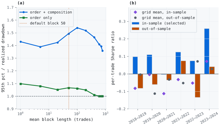
Figure 2. 2-panel illustration of block-length sensitivity and walk-forward degradation

• Panel (a): the ratio of the 95th-percentile drawdown to the realized drawdown against mean block length, from 1 to 780 trades on the 820-trade series. With order and composition varied (blue), the ratio is between 1.39 and 1.54 for blocks of 1 to 100, peaks at 1.54 at a block of 100, and declines to 1.36 at 780. With order alone varied (green), it is 1.10 at a block of 1 and reaches 1.00 from a block of 600 on.
• Panel (b): paired in-sample and out-of-sample per-trade Sharpe ratio for each of six annual walk-forward windows, with the average over all 16 grid points in each period shown as markers. The in-sample step is a 4×4 grid search over the long-entry and short-entry RSI thresholds (20 to 35 and 65 to 80), refit every year. Out-of-sample performance is lower than in-sample performance in all six windows.

Panel (a) does not confirm the short-block failure on this series, and it should not be read as if it did. The ratio's denominator is a single realized drawdown, so the ratio inherits that draw's noise. As a check, the trade order was shuffled 40 times, which removes any real dependence, and the ratio was recomputed at blocks of 1 and 100. On the real order, the ratio at block 100 exceeds the ratio at block 1 by 0.11. On shuffled orders the same difference ranges from −0.78 to 0.30 (5th to 95th percentile), so 0.11 is not distinguishable from what independent trades produce.

At the long-block end, the blue curve does not approach 1.0 within the range tested, since a geometric block with a mean of 780 trades still splits most replicates into more than one randomly placed block. In the single-block limit every replicate is a rotation. On this series no rotation of the 820 trades has a deeper drawdown than the realized path, and 51% of the rotations leave the worst stretch intact, so the limit here is 1.0. That is a property of this series and not a general result.

The practical reading is the range. Across every block length tested, varying order and composition puts the 95th-percentile drawdown between 1.36 and 1.54 times the realized one; varying order alone puts it between 1.00 and 1.10 times. Reporting those bands is more informative than reporting the value at any one block.

The serial-dependence checks from Section 4 show where dependence does exist. A Ljung-Box test on the trade returns gives raw p-values between 0.26 and 0.90 at every lag from 1 to 20, so there is no evidence of autocorrelation in the returns before any adjustment. On their absolute values the raw p-value is 0.083 at lag 1, and after Holm adjustment across the twenty lags the p-value is at most 0.007 at every lag from 2 to 20. The sign of a trade is not predictable from its neighbors, but its size is, and a block longer than one preserves that clustering of magnitudes.

Is the trade distribution stationary?

Both resampling schemes treat the seven years as draws from one distribution. Per-year summaries of the trade returns, in basis points of account equity:

Year	Trades	Mean (bp)	Std. dev. (bp)
2018	126	4.1	41.4
2019	105	−2.5	30.2
2020	121	−7.0	35.7
2021	113	0.1	27.3
2022	113	−0.5	58.9
2023	119	3.7	41.9
2024	123	4.4	33.1

A Brown-Forsythe test of equal spread across the seven years rejects it (p < 0.001), while a Kruskal-Wallis test finds no evidence of a shift in location (p = 0.21). The size of the trades is not stationary: the standard deviation in 2022 is more than twice that in 2021. The resampling mixes years in proportion to their trades, so the tail it reports is an average over the regimes in the sample, not a forecast for any one of them.

The sensitivity is large. Resampling only the 352 trades of 2018 through 2020 (mean −1.7 bp per trade, standard deviation 36.5 bp), 5.68% of one-year paths breach a static 10% floor, with a 95% Monte Carlo interval of [5.54%, 5.83%]. Resampling only the 468 trades of 2021 through 2024 (mean 2.0 bp, standard deviation 41.8 bp), the fraction is 0.006% [0.002%, 0.013%]. The full-sample figures below sit between these, and they implicitly weight the two regimes by their share of the sample.

Breach probability on trades and on calendar days

The fraction of paths that breach a limit needs two qualifications before it says anything about a funded account. The first is horizon: a seven-year fraction is not comparable with a one-year evaluation. The second is the rule's basis. The FundedNext floor is static. The lowest point of the realized equity curve at trade exits is 91.25% of the starting balance, so the realized path passes that rule even though its peak-to-trough drawdown of 14.3% exceeds 10%. Trade-level estimates, from 100,000 resampled paths each, with 95% Monte Carlo intervals for the one-year horizon of 117 trades:

Limit and basis	Realized path	Breach, 1-year paths	Breach, 7-year paths
10%, static	Passes	1.45% [1.38%, 1.53%]	27.7%
10%, trailing	Breaches	2.22% [2.13%, 2.31%]	56.3%
15%, static	Passes	0.027% [0.018%, 0.039%]	11.4%
15%, trailing	Passes	0.040% [0.029%, 0.054%]	22.8%

The same rules checked on floating equity, with server days resampled in blocks of 111 days (the 50-trade block expressed in days) and a one-year horizon of 260 server days. The daily row applies the 5% daily limit to every path in the other rows:

Limit and basis	Realized path, floating	Breach, 1-year paths	Breach, 7-year paths
10%, static	Passes	1.72% [1.64%, 1.80%]	28.9%
10%, trailing	Breaches	2.86% [2.76%, 2.96%]	58.9%
15%, static	Passes	0.027% [0.018%, 0.039%]	12.3%
15%, trailing	Passes	0.044% [0.032%, 0.059%]	24.6%
5%, daily	Passes (worst day 2.11%)	0% [0%, 0.004%]	0%

Moving from exit-only trade paths to floating equity on calendar days raises seven of the eight overall-limit estimates, for example from 1.45% to 1.72% of one-year paths for the static 10% floor, and leaves the one-year static 15% estimate unchanged. Two things change at once, the equity measured and the resampling unit, so the difference should not be attributed to floating equity alone. The direction agrees with the warning in Section 5: exit-only checks can understate, and cannot overstate, rules applied to floating equity.

The daily limit

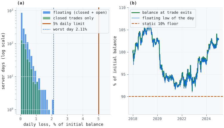
Figure 3. 2-panel illustration of the calendar-day check on the realized path

• Panel (a): the daily loss on each of the 1,821 server days, measured from the balance at midnight as a percentage of the initial balance, on floating equity (blue) and on closed trades only (green, days with a closed loss). The vertical axis is logarithmic. The worst day loses 2.11% on floating equity against a 5% limit.
• Panel (b): the closed balance at trade exits and the lowest floating equity of each day, against the static floor at 90% of the initial balance. The lowest floating point is 90.97% of the initial balance, against 91.25% at exits.

The trade-level check with trades_per_day=1 finds no breach of the 5% daily limit in 100,000 one-year paths, but that grouping alone does not justify the conclusion. On the calendar, 818 server days have one exit, one day has two, and 1,002 days have none, so one trade per day is close to the calendar for this strategy. What the grouping misses is the open position: the largest single-trade loss is 1.30%, the worst closed-trade day loses 1.23% of the initial balance, and the worst day on floating equity loses 2.11%.

No resampled calendar path breaches the daily limit either, and the Monte Carlo upper bound is 0.004% of paths. As Section 5 explains, that zero is not independent evidence, because day resampling cannot create a day worse than the worst observed one. The supportable statement is narrower. On this quote history, at one times notional, the worst server day on floating equity used less than half of the 5% daily limit, and the overall floor is the binding rule.

These are statements about resampled paths under the same-distribution assumption, not forecasts of a live account. They also hold only at one times notional, and they do not scale in proportion to leverage, because losses compound on a shrinking base and a limit is crossed or not. At two times notional, the realized drawdown is 27.0% rather than twice 14.3%, the 95th percentile is 38.6%, and 16.2% of one-year trade paths breach the static 10% floor, against 1.45% at one times. At three times the figures are 38.2%, 52.6% and 31.6%.

Walk-forward degradation

The walk-forward result needed no adversarial construction. It is what a 4×4 grid search over two thresholds does on ordinary annual refits. The score is the per-trade Sharpe ratio (the mean trade return divided by its standard deviation, not annualized). Mean in-sample score across the six windows is 0.111, and mean out-of-sample score is −0.033. The paired degradation is 0.144, with a 90% bootstrap interval of [0.091, 0.196], so result.degrades is True.

That interval adds less than it appears to. Every window degraded, so no bootstrap mean can fall at or below zero, and the interval excludes zero as a consequence of the sign pattern. Six windows are a thin base, and the primary evidence is the count itself: six degraded windows out of six give a one-sided sign-test p-value of 1/64, about 0.016, under the null that degradation is equally likely to be positive or negative in independent windows. The windows are not fully independent, since each out-of-sample year is the next window's in-sample year, so even that figure is approximate. Repeating the study with half-year windows gives 13 windows, of which 12 degraded (sign-test p = 0.0017), with a mean degradation of 0.206 [0.144, 0.268]. The half-year windows reuse the same seven years, so they are not independent confirmation; they show only that the result does not hinge on the window length.

The traditional WFE ratio on the six annual windows is −0.29. wfe_reliable is False because the 2020 in-sample window is slightly negative (−0.004), so the denominator averages scores of opposite sign. Following the rule in Section 6, its magnitude is not interpreted here. Its negative sign says only what the means already say, that the selected thresholds lost money out of sample while scoring positively in sample.

Positive degradation does not by itself say why. To separate selection from a change that affects every candidate, each window's degradation splits into three terms. The first is the in-sample advantage of the selected thresholds over the average of the 16 grid points, which averages 0.146. The second is the change in the grid average from in-sample to out-of-sample: the average rose from −0.035 to −0.017, so this term is −0.019. The third is the out-of-sample shortfall of the selected thresholds against the grid average, 0.016. The in-sample selection premium alone is slightly larger than the whole degradation of 0.144, and the grid as a whole did not deteriorate out of sample. The half-year windows show a similar split: a selection premium of 0.180 out of a degradation of 0.206, and a change in the grid average of 0.008.

This decomposition is consistent with selection from a family with no detectable edge, and with about 100 trades per year the standard error of a per-trade Sharpe estimate is roughly 0.1, so a gap of this size is within what selecting the best of 16 noisy estimates can produce. It does not prove that selection is the only cause. A change that hurt only the selected thresholds would leave the same footprint, and six windows cannot rule it out. Six windows and a 4×4 grid also cannot distinguish no edge from a small edge, and this section is not a verdict on RSI mean reversion. Part 26 tests the related question directly, by rerunning the whole search on permuted data rather than watching it degrade one period at a time.

Conclusion

The path a backtest took is one draw from the paths its trades could have produced, and treating it as a fixed property of the strategy misstates risk. The conclusions fall into two groups.

Methodological conclusions

These hold for any trade series and do not depend on the attached data:

• Report the resampled tail alongside the realized drawdown, and say what it measures. The stationary bootstrap varies order and composition together; the block permutation varies order alone.
• Treat the block length as an assumption and report the band. suggested_block_length is a starting point for overlapping labels, and for non-overlapping trades it returns its floor. Test returns and absolute returns for serial dependence with a correction across lags, then report how the tail moves across block lengths.
• Match the rule, not just the limit. A prop-firm limit has a basis, a horizon, a clock and an equity definition. Checks at trade exits with trades grouped by count can understate rules applied to floating equity on calendar days.
• Attach a Monte Carlo interval to every rare breach probability. An estimate based on a handful of breaching paths is not stable without one.
• Report the paired difference with the sign count. The WFE ratio answers a relative question; the paired difference states the loss in score units.
• Decompose degradation before naming a cause. Compare the selected candidate with the average unselected one in both periods.

Results specific to this data set

These hold for the attached EURUSD file, this RSI rule, the spread as the only cost and one times notional:

• The 95th-percentile drawdown is 21.4% against a realized 14.3%, a ratio between 1.36 and 1.54 across block lengths. With order alone varied, the ratio is between 1.00 and 1.10.
• The sampling uncertainty of that tail is wide: 8.6% to 32.0% for the 95th percentile.
• Trade size is not stationary across years, and the one-year static-floor breach fraction ranges from 0.006% to 5.68% depending on which half of the sample is resampled.
• The realized path passes the static 10% floor; 1.72% of one-year calendar paths on floating equity fail it. The worst server day lost 2.11% of the initial balance on floating equity, against a 5% daily limit.
• All six annual walk-forward windows degraded, and the in-sample selection premium is as large as the degradation while the average grid point did not deteriorate.

Part 25 asks the question none of this article's tools address: once a strategy is deployed, how would you know from the trade stream itself that it had stopped working, without either reacting to normal variance or missing a real deterioration for months?

Attached Files

	File	Module	Description
1.	bootstrap.py	afml.backtest_statistics	block_permutation_indices, max_drawdown, bootstrap_statistic, bootstrap_drawdown_distribution, sequence_risk_ratio, breach_probability, binomial_mc_interval, quantile_mc_interval.
2.	calendar.py	afml.backtest_statistics	mark_to_market_days, realized_account_checks, calendar_breach_probability.
3.	walkforward.py	afml.backtest_statistics	DegradationResult, walkforward_degradation.
4.	Files from the previous version of the project: screening/ (10 files) and codependence/ (5 files)	afml.screening, afml.codependence	The package from Part 23. Supplies stationary_bootstrap_indices and suggested_block_length; afml.codependence is required by afml.screening on import.
5.	test_bootstrap_evaluation.py	afml.tests	Unit tests for the three modules.
6.	part24_reproduce.py	Script	Reproduces every number in Section 7 from the data file and writes them to a JSON file.
7.	generate_figures.py	Script	Draws Figures 1 to 3 from the data file and the JSON output of part24_reproduce.py.
8.	EURUSD_H1_time_2018-01-01-2024-12-31.parq	Data	The EURUSD H1 bid and ask bars described in Section 2.

Further Reading

• Brown, M. B., & Forsythe, A. B. (1974). Robust tests for the equality of variances. Journal of the American Statistical Association, 69(346), 364–367.
• Clopper, C. J., & Pearson, E. S. (1934). The use of confidence or fiducial limits illustrated in the case of the binomial. Biometrika, 26(4), 404–413.
• FundedNext Help Center. Daily Loss Limit vs Overall Loss Limit and How can I calculate the daily loss limit? Accessed October 2026.
• Holm, S. (1979). A simple sequentially rejective multiple test procedure. Scandinavian Journal of Statistics, 6(2), 65–70.
• Kruskal, W. H., & Wallis, W. A. (1952). Use of ranks in one-criterion variance analysis. Journal of the American Statistical Association, 47(260), 583–621.
• Ljung, G. M., & Box, G. E. P. (1978). On a measure of lack of fit in time series models. Biometrika, 65(2), 297–303.
• López de Prado, M. (2018). Advances in Financial Machine Learning. John Wiley & Sons.
• Masters, T. (2020). Permutation and Randomization Tests for Trading System Development.
• Pardo, R. (2008). The Evaluation and Optimization of Trading Strategies (2nd ed.). John Wiley & Sons.
• Politis, D. N., & Romano, J. P. (1994). The stationary bootstrap. Journal of the American Statistical Association, 89(428), 1303–1313.