Machine Learning in Pure MQL5 (Part 1): Logistic Regression from Scratch with SGD

Contents

1. Why pure MQL5, and what this series is
2. The problem logistic regression solves
3. The three formulas behind it
4. From price to a probability
5. The class: a dependency-free CLogReg
6. Standardizing the features without leakage
7. Learning by stochastic gradient descent
8. Turning price into features
9. The honest test: train here, measure there
10. Reading the result: a faint edge, and a warning
11. Files and how to run it
12. Limitations
13. What Part 2 adds
14. Conclusion

Why pure MQL5, and what this series is 

There is no shortage of machine learning on this site, but almost all of it leans on something outside the terminal: a Python bridge, an ONNX runtime exported from scikit-learn or PyTorch, an external library pulled from a repository. That is fine until you want to run the thing on a plain VPS with nothing installed, or ship it to someone who does not have your toolchain, or simply understand what the model is actually doing instead of treating it as a black box behind an import.

This series takes the other road. Every model in it is written from scratch in 100 percent native MQL5: no Python, no ONNX, no DLL, no third-party library, and not even the built-in matrix type. Just double arrays and arithmetic you can read line by line. The result is a small, dependency-free machine learning library that compiles anywhere MQL5 does and that you own completely. The most complete existing series on the topic is the Data Science and Machine Learning series. It starts from scratch, moves to the matrix type by Part 3, and uses Python and ONNX in later parts. It also packages the code as an external repository. This series holds the opposite line the whole way: nothing installed, nothing imported, the code is the deliverable.

Part 1 is the foundation, and it is deliberately the simplest useful model there is: logistic regression, which is nothing more than a single neuron. Everything later in the series, up to a small neural network, is built from the pieces we lay down here. This is a teaching and tooling article, not a trading system, and it makes no promise of profit.

The problem logistic regression solves

Logistic regression answers a yes or no question with a probability. Given a handful of numbers describing the current state of the market, it outputs a single number between zero and one: the probability that some event happens. Here the event is simple and honest to test, the next bar closes higher than this one. Feed the model the present, and it returns its estimated probability that the next candle is green.

It does this with a straight line through the inputs, squashed into the zero-to-one range. Each input feature gets a weight, the weighted inputs are added up with a bias term, and that sum is passed through a function that bends any real number into a probability. Training is the process of finding the weights that make those probabilities line up with what actually happened in history. That is the whole idea, and the three formulas below are all of the mathematics involved.

The three formulas behind it

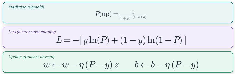
The entire model, in three lines. The sigmoid turns a weighted sum into a probability, the loss measures how wrong that probability was, and the update nudges the weights to be less wrong next time.

The first formula is the sigmoid. It takes the weighted sum of the inputs and returns a probability, gently for inputs near zero and saturating toward one or zero for large positive or negative sums. The second is the loss, binary cross-entropy, which is large when the model is confidently wrong and near zero when it is confidently right. The third is the update rule, and it hides a small piece of good luck: the gradient of the cross-entropy loss with respect to the weights turns out to be simply the error, the predicted probability minus the true label, times the input. There is no messy derivative to code. The error itself tells each weight how to move.

From price to a probability

Before any code, it helps to see the path a single bar takes through the model, because the class does exactly this and nothing more.

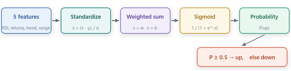
Five raw features are standardized, combined into one weighted sum, squashed by the sigmoid into a probability, and thresholded into a class. Each box is a step you will find in the code.

Raw features come in on the left. They are put on a common scale by standardization, combined into a single number by the weighted sum, and turned into a probability by the sigmoid. A threshold of 0.5 converts that probability into a hard call, up or down. The interesting engineering is in two of those boxes, the standardization and the training that sets the weights, and the rest of the article is those two boxes in native code.

The class: a dependency-free CLogReg

The deliverable is one file, `LogReg.mqh`, holding one class. Nothing else is required, no include beyond it, no library. Here is the heart of inference, the sigmoid and the prediction, so you can see there is no magic under the hood.

   //+------------------------------------------------------------------+
   //| Sigmoid: numerically stable logistic function                    |
   //+------------------------------------------------------------------+
   double   Sigmoid(const double z)
     {
      if(z >= 0.0)
         return(1.0 / (1.0 + MathExp(-z)));
      double e = MathExp(z);              // stable form for very negative z
      return(e / (1.0 + e));
     }

The sigmoid is written in two branches on purpose. The naive form is numerically unstable for large-magnitude inputs, so for negative sums we use the algebraically identical form that never exponentiates a large positive number. Prediction then standardizes the incoming row, forms the weighted sum, and passes it through that sigmoid.

//+------------------------------------------------------------------+
//| Probability of class 1 for a raw feature row.                    |
//+------------------------------------------------------------------+
double CLogReg::Predict(const double &raw[])
  {
   double z[];
   Standardize(raw, z);
   double s = m_b;
   for(int j = 0; j < m_nf; j++)
      s += m_w[j] * z[j];
   return(Sigmoid(s));
  }

That is the entire forward pass. A prediction is a dot product of weights and standardized features, plus a bias, run through the sigmoid. The rest of the class exists to find good values for those weights.

Standardizing the features without leakage

Features on different scales, an oscillator that lives between minus and plus a half next to a return measured in ATR units, will confuse gradient descent unless they are first put on a common footing. Standardization subtracts each feature's mean and divides by its standard deviation, so every feature arrives centered at zero with unit spread. The subtle part is not the arithmetic, it is where the mean and standard deviation come from.

//+------------------------------------------------------------------+
//| Compute per-feature mean and stdev over the training rows.       |
//| Fitting the scaler on TRAIN ONLY avoids look-ahead leakage.      |
//+------------------------------------------------------------------+
void CLogReg::FitScaler(const double &X[], const int rows)
  {
   for(int j = 0; j < m_nf; j++)
     {
      double s = 0.0;
      for(int i = 0; i < rows; i++)
         s += X[i * m_nf + j];
      double mean = s / rows;
      double v = 0.0;
      for(int i = 0; i < rows; i++)
        {
         double d = X[i * m_nf + j] - mean;
         v += d * d;
        }
      double sd = MathSqrt(v / rows);
      if(sd < 1e-12)
         sd = 1.0;               // a constant feature: leave it untouched
      m_mean[j] = mean;
      m_std[j]  = sd;
     }
   m_scaled = true;
  }

The scaler is fitted on the training rows only, and then the same fixed means and deviations are applied to the out-of-sample rows. Computing them over the whole history instead, including the part you will later test on, leaks information from the future into the past and quietly inflates the result. This is the most common way to introduce look-ahead leakage in market ML. Avoiding it requires a single choice: fit the scaler only on the training rows you pass to this function.

Learning by stochastic gradient descent

Training walks through the training examples one at a time, and for each one it makes a prediction, measures the error, and nudges every weight a little in the direction that would have reduced that error. One pass over all the rows is an epoch, and the rows are shuffled each epoch so the model does not learn an accidental order.

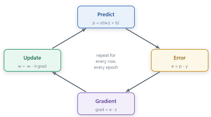
The training loop. Predict, measure the error, form the gradient, update the weights, and repeat for every row of every epoch.

      loss = 0.0;
      for(int t = 0; t < rows; t++)
        {
         int i = order[t];
         //--- standardize this row
         for(int j = 0; j < m_nf; j++)
            z[j] = (X[i * m_nf + j] - m_mean[j]) / m_std[j];
         //--- forward pass
         double s = m_b;
         for(int j = 0; j < m_nf; j++)
            s += m_w[j] * z[j];
         double p = Sigmoid(s);
         //--- gradient of cross-entropy is simply (p - y)
         double err = p - (double)y[i];
         //--- update weights and bias
         for(int j = 0; j < m_nf; j++)
            m_w[j] -= m_lr * err * z[j];
         m_b -= m_lr * err;
         //--- accumulate loss for reporting
         double pc = MathMax(1e-12, MathMin(1.0 - 1e-12, p));
         loss += -(y[i] * MathLog(pc) + (1 - y[i]) * MathLog(1.0 - pc));
        }

This inner loop is the whole learner. The prediction is formed exactly as in `Predict`, the error is the probability minus the label, and each weight moves by the learning rate times that error times the corresponding input. The last two lines only track the cross-entropy loss so training can be reported, they do not change the model. There is no library call, no matrix inversion, no gradient framework. It is arithmetic in a loop, and it is enough to fit a logistic regression to as many bars as you care to give it. The learning rate controls the step size. If it is too large, the weights oscillate; if too small, training is slow. The default value (0.05) is a reasonable middle ground for standardized inputs.

Turning price into features

A model is only as good as what you feed it, and the demo keeps the inputs deliberately plain and native: five numbers computed from standard indicators, each normalized so it means the same thing across instruments and eras.

      double a = atr[k];
      if(a <= 0.0)
         continue;
      //--- five simple, native, standardizable features
      double f0 = rsi[k] / 100.0 - 0.5;                       // momentum oscillator, centered
      double f1 = (r[k].close - r[k-1].close) / a;            // last return, ATR-normalized
      double f2 = (r[k].close - r[k-5].close) / a;            // 5-bar return, ATR-normalized
      double f3 = (r[k].close - ema[k]) / a;                  // distance from trend, ATR-normalized
      double f4 = (r[k].high - r[k].low) / a;                 // bar range, ATR-normalized
      //--- label: did the NEXT bar close up?
      int label = (r[k+1].close > r[k].close) ? 1 : 0;

Dividing the returns and the range by the ATR is what makes a feature computed on gold comparable to the same feature on the euro: it measures movement in units of the instrument's own recent volatility rather than in raw price. The label looks exactly one bar into the future, which is the only place a label is ever allowed to look.

The honest test: train here, measure there

The demo pulls about 40,000 hourly bars, builds the feature matrix and the labels, and splits the history in two. The first 70 percent is the training block, roughly 28,000 rows, where the scaler is fitted and the weights are learned over 200 epochs. The last 30 percent, about 12,000 rows the model has never seen, is the out-of-sample block where the only number that counts is measured. Alongside the model's accuracy we compute a baseline, the accuracy you would get by always predicting the majority class of the training block, because a model that cannot beat that dumb rule has learned nothing worth having.

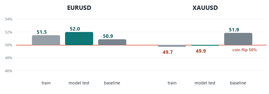
Out-of-sample accuracy on two instruments, next to the coin flip and the majority-class baseline. On EURUSD the model edges the baseline; on XAUUSD it does not.

Reading the result: a faint edge, and a warning

On the euro, the model scored 52.0 percent on the out-of-sample bars against a majority baseline of 50.9 percent, and within the top 10 percent of predictions by confidence, accuracy rose to 53.9 percent. That is a faint edge, a little above the coin flip and a little above the baseline, and the fact that confidence and accuracy move together is a small sign the model found something real rather than noise.

On gold, the same model scored 49.9 percent out-of-sample against a baseline of 51.9 percent. Read that carefully: the model did worse than simply betting on the majority class every time. With these five naive features, it underperformed the dumbest possible rule. This is the warning the whole article is built to deliver. A model can look busy, produce weights, and draw a confident-looking probability for every bar, and still carry no edge at all. The only way you find out is the honest split and the baseline, and here they say plainly that logistic regression on these particular features extracts a little on the euro and nothing on gold.

The difference between the two instruments shows the risk of cherry-picking results. Had the demo run on ten symbols and reported only the euro, it would read as a success story, when the honest picture is one faint edge among results that hover around a coin flip. The training accuracy tells the same story from another angle: at 51.5 percent on the euro it is barely above the out-of-sample figure, which is what you want to see, because a training score far above the test score is the signature of a model that memorized noise rather than learning a pattern. When training and test accuracy are close to each other and close to the baseline, it indicates a weak signal rather than overfitting. That is not a disappointing result to hide, it is the correct result to report, and it is the discipline every later part of this series will keep.

Files and how to run it

The library is one include file; the demo is one script that uses it.

File	What it holds
LogReg.mqh	The dependency-free logistic regression class: standardization, sigmoid, prediction, SGD training, and save/load of a trained model. This is the reusable deliverable.
LogRegDemo.mq5	A script that builds native features, labels the next-bar direction, splits in-sample and out-of-sample, trains, and reports honest accuracy plus a per-row CSV.

To reproduce the numbers:

1. Put both files in the same MQL5\Scripts folder and compile the script; the include is picked up automatically.
2. Drag the script onto the chart of the symbol and timeframe you want, and keep the defaults or adjust the periods.
3. Read the accuracy, the baseline, and the confusion matrix in the Experts tab, and find the per-row predictions written to the shared Files folder as a CSV.

Limitations

1. The features are deliberately basic. Better features would matter far more than a fancier model, and later parts explore both.
2. Logistic regression is linear in its inputs, so it cannot capture interactions between features. That is a reason to move to richer models later, not a defect here.
3. Next-bar direction is a hard, nearly balanced target. A faint edge is the realistic outcome, and any result far above the coin flip on this target should be treated as a bug or leakage until proven otherwise.
4. Accuracy is not profit. Being right slightly more than half the time says nothing about the size of the moves you catch versus the ones you miss, which is a separate measurement.
5. Results are from one broker's history over one period per symbol. Reproduce them on your own data before trusting them.

What Part 2 adds

Part 1 leaves you with a working, dependency-free classifier and, more importantly, the scaffolding every model needs: features, standardization without leakage, an honest split, and a baseline. Part 2 reuses all of it and swaps the model, keeping the exact same evaluation so the comparison is fair. The pieces here, the sigmoid, the loss, and the gradient step, are also literally one neuron, which is the reason logistic regression is the right place to start a series that ends in a network of them.

Conclusion

Logistic regression is the smallest honest machine learning model, and written in pure MQL5 it is about a hundred lines with no dependencies of any kind. Building it from scratch shows there is nothing mystical inside: a weighted sum, a squashing function, and an update rule that is just the error times the input. The harder and more valuable half is the evaluation, and it gave an uncomfortable but honest verdict, a faint edge on the euro and less than nothing on gold, which is exactly the kind of result you want your testing to be able to tell you. The model is the easy part. Measuring it without fooling yourself is the craft, and it is the through-line of this series.

A final note: this is an educational article, not financial advice, and nothing here is a promise of profit. The value is the reusable native code and an honest way to judge it.