

Neural Networks in Trading: Heterogeneity-Informed Meta-Parameter Learning (HimNet)
 157
157
 0
0

Introduction
The emergence of a wide range of tools for collecting streaming data has led to the large-scale accumulation of spatio-temporal series in a wide variety of areas of human activity. Trading systems generate streams of quotes, orders, and trades across different trading venues, tickers, and instrument types. As data volumes grow, accurate forecasting of such series becomes a tool for reducing costs, managing risks, and improving the execution of trading strategies. An error in forecasting local liquidity or volatility directly results in slippage, lost profits, and distorted performance metrics for a trading strategy. Therefore, a high-quality model must account not only for global trends but also for local, context-specific differences: where and when the market is tight, and where it is loose.
The key challenge is the spatio-temporal heterogeneity of the data. Spatial heterogeneity in the market manifests itself when different trading venues or assets exhibit different patterns at the same time. For example, some exchanges may have deep liquidity, while others may have arbitrage gaps, especially during periods of high volatility. Under these conditions, attempting to average the behavior of all trading venues leads to the smoothing out of important local effects and a loss of accuracy.
Temporal heterogeneity is more pronounced than it appears at first glance. The behavior of the same financial instrument varies dramatically at different times of the day and on different calendar dates. The opening and closing of a trading session are two striking examples: in the first few minutes after the opening, there is a surge in volume and volatility, while late in the evening, on the contrary, activity is low. News and macro announcements trigger short-term regimes of extreme volatility. Holidays and weekends lead to a lull in activity. Taken together, this means that the same pattern cannot be considered stationary over time — its statistics change, and the model must take this into account.
Previously proposed approaches have attempted to address the problem in various ways, but each has its limitations when it comes to practical application in trading. Graph-based methods relied on topology and precomputed similarity metrics between data points — much like a trader who bases their strategy entirely on a liquidity map drawn in advance. In the real world, the map quickly becomes outdated: the composition of market makers changes, new trading venues emerge, and temporary liquidity gaps occur.
Meta-learning methods provided the idea of storing multiple sets of parameters for different regimes, but often required external information. In finance, this means that accessible and accurate metadata is needed for each trading venue and instrument. But it is not always possible to obtain it in real time. In addition, many of these approaches are too memory-intensive and computationally expensive.
Representation-based approaches (Representation Learning) have learned to extract informative embeddings from raw data. This is powerful, but it is often followed by simplified processing of the embeddings, and the value of a good representation is lost in the next step. Self-Supervised learning adds auxiliary tasks to make the embeddings richer — this is useful, but it does not always allow the model to be trained optimally for the target forecasting task within a single cycle.
That is precisely why the authors of the paper "Heterogeneity-Informed Meta-Parameter Learning for Spatiotemporal Time Series Forecasting" proposed a different approach — the HimNet framework. Their solution combines two key components. First, heterogeneity is identified implicitly through trainable spatial and temporal embeddings, and then this information is used for meta-parameter learning of the model parameters. Simply put, the framework's creators not only aim to identify differences between individual data segments, but also train the model to select and generate unique parameters for each context.
Imagine that the pool of trading information contains:
- shares of the largest issuer on the main exchange during business hours;
- the same stocks on over-the-counter trading venues following a local news spike;
- small-cap securities with low liquidity;
- crypto markets with varying order book depths.
Spatial embeddings will separate these groups into distinct clusters. The system then retrieves a dedicated parameter set for each cluster from the meta-parameter pool: aggressive settings for the main market that take low slippage into account, conservative ones for OTC trading to increase the execution safety margin, broader regularization for small-cap securities to avoid overfitting to noise, and a noise-aware configuration for crypto for high noise levels and frequent arbitrage gaps. All of this is trained in a single cycle, so the model learns to distinguish between contexts and select the best parameters for them simultaneously.
Temporal examples are just as important. The morning market open often requires a quick response and short-term volume forecasts. The periods following the release of key macroeconomic data are a heightened-volatility regime. The late hours are a low-activity regime. The meta-parameter mechanism proposed by the framework's authors can allocate separate parameter sets for temporal regimes. It is similar to how an experienced trader adjusts their trading style depending on the time of day and the calendar.
Technically, the key idea is to cluster embeddings and dynamically quantize parameters through a small, computationally efficient pool of meta-parameters. This solves several problems with previous approaches at once. First, there is no strict dependence on external auxiliary features — the model identifies relevant contexts on its own. Second, the pool of meta-parameters is compact, so memory and computational resource usage remain manageable, which is important for systems requiring low execution latency. Third, the framework's authors move from passively identifying heterogeneity to actively using it: clusters directly determine which parameters are applied. This increases the accuracy of forecasts and improves the quality of execution.
Interpretability deserves a special mention. Meta-parameters and clusters can be visualized: a cluster map will show which trading venues and which time windows belong to the same regime; a heatmap of meta-parameters will illustrate how the settings differ between low- and high-volatility regimes. For practitioners, this is not just a nice chart but also a monitoring tool: if a cluster unexpectedly includes trading venues that are fundamentally different, this is a signal to perform additional data validation or review the preprocessing procedure.
Finally, robustness and transferability. An important feature of the HimNet framework is its flexibility across domains. Meta-parameters and embeddings are trained so that they can be applied to other instruments and trading venues with minimal fine-tuning.
Ultimately, the HimNet framework offers a practical and effective way to identify spatio-temporal regimes, forms a compact pool of meta-parameters, and trains the model to use the information obtained. This provides traders and developers of forecasting systems with a tool that simultaneously improves accuracy, maintains computational efficiency, and enhances interpretability.
The HimNet Algorithm
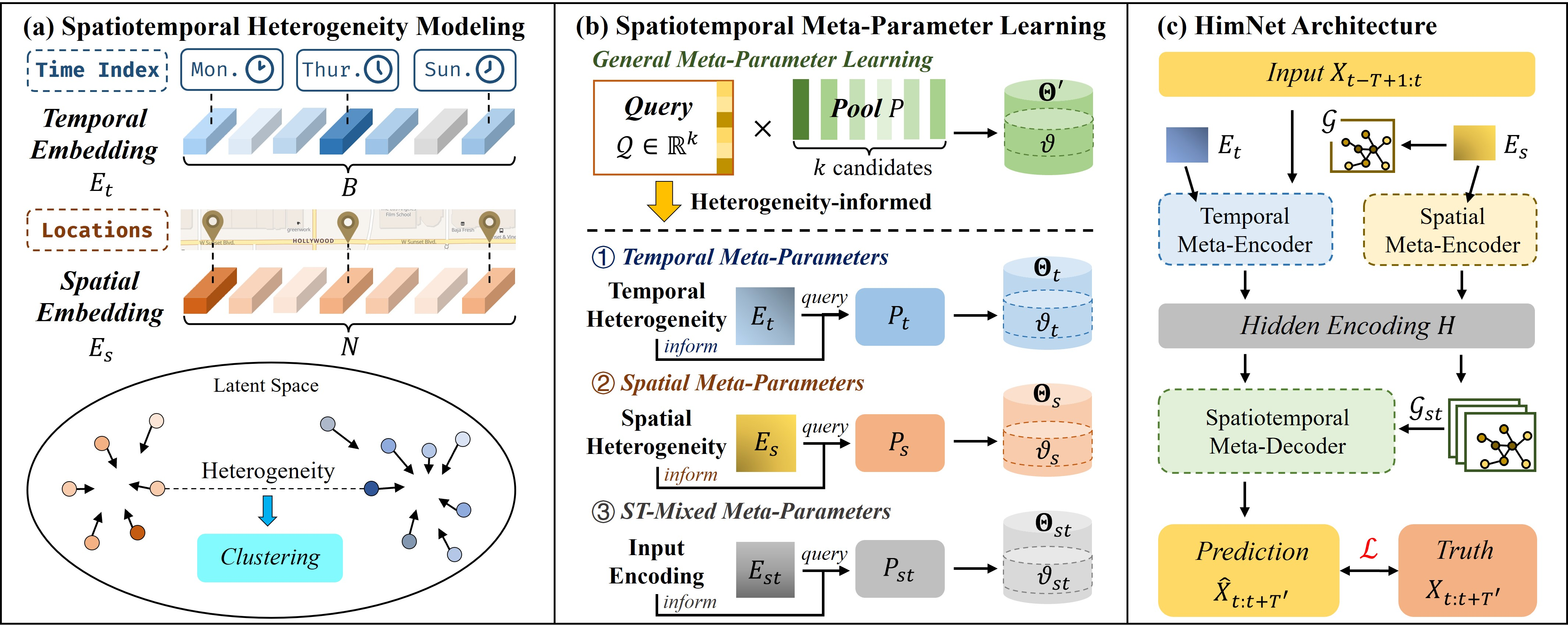
A key aspect of modeling spatio-temporal heterogeneity is correctly identifying and separating the source-data context along the temporal and spatial dimensions. Instead of using external reference data, the authors of the HimNet framework create trainable embeddings that assign a unique representation to each spatio-temporal context. This gives the model the flexibility and adaptability needed to solve real-world financial problems.
For the temporal dimension, the framework's authors create two embedding dictionaries:
- time-of-day dictionary Dtod ∈ RNd × dtod;
- day-of-week dictionary Ddow ∈ RNw × ddow.
Here, dtod and ddow are the dimensions of the corresponding vectors, Nd is the number of steps within a trading day, and Nw is the number of days in a week.
For a mini-batch of input data Xb ∈ RB×T×N with history length T, the framework authors propose using the timestamp of the last step of each sample to select temporal embeddings Etod ∈ RB×dtod and Edow ∈ RB×ddow from the dictionaries. They then concatenate them into a shared temporal embedding.

The practical rationale for this separation is simple. Time of day captures high-resolution periodicity: morning spikes at the open, a midday lull, and the evening session. The day of the week captures longer cycles: behavior on weekdays and weekends, as well as recurring patterns around reporting dates and economic releases. Together, these dictionaries enable the model to recognize temporal regimes across multiple scales and select appropriate forecasting parameters for them.
For the spatial dimension, the authors of the framework use a spatial embedding matrix Es ∈ RN*ds, where N is the number of time series or locations, and ds is the vector dimension for each location. Unlike temporal dictionaries, here each spatial element is directly associated with its own learnable vector, which is initialized randomly. The goal is to capture the functional differences between trading venues that affect time-series patterns: order book depth, execution speed, participant profiles, instrument types, and infrastructure characteristics. This makes it possible to account for spatial heterogeneity without explicitly using auxiliary features.
This type of embedding training essentially performs dynamic clustering. During training, the representations in the matrices gradually diverge and cluster depending on the input data. Embeddings associated with spatio-temporal contexts that exhibit similar behavior move closer together in the latent space. Those with different dynamics diverge. As a result, natural clusters emerge — typical behavioral regimes. This is similar to language models, where king and queen turn out to be semantically close. Only here, closeness reflects the similarity of market regimes. Importantly, this clustering emerges organically, without rigid external constraints or manual labeling. The model learns on its own which contexts are similar and which are not.
Let us examine some financial examples in more detail to show more concretely how this works in practice. Let us consider a few typical contexts:
- The opening of the main stock market session. High activity, large volumes, rapid price fluctuations. For such temporal and spatial combinations, the model will identify a specific embedding and select parameters geared toward short horizons and rapid response — this is important for fast-execution algorithms and reducing slippage.
- Over-the-counter trading in the same securities during the night. Low volumes, infrequent trades, and an increased risk of sharp price swings caused by isolated orders. Here, the temporal embeddings will differ, and the meta-parameters will make the model more conservative, increasing robustness and reducing the likelihood of overfitting to noise.
- Cryptocurrency exchanges with varying order book depths. One exchange has deep liquidity, while another has thin liquidity and an arbitrage profile. Spatial embeddings will separate these trading venues, and the model will apply different strategies for forecasting volume and price, which is useful for arbitrage systems.
- Days of major macro releases or quarterly earnings reports. Temporal embeddings for the day of the week, together with the time of day, will identify such windows; the model will switch to a regime with increased sensitivity to short-term signals and wider confidence intervals.
The key idea is simple yet effective. Our task is not only to capture heterogeneity, but also to learn how to control it. To make it practically useful for forecasting and execution in the markets. Instead of trying to maintain a separate set of parameters for every minute and for every exchange — which is economically and technically untenable — the framework’s authors extend the model’s parameter space along the temporal and spatial dimensions, and then compactly represent this extension as small pools of meta-parameters. For a specific spatio-temporal query, the final parameters are generated as a weighted combination of candidates from the pool: Θ = Q · P. This approach allows us to work with a compact set of parameters rather than optimizing a vast number of unique ones, which drastically reduces memory and computational requirements. Instead of paying for scaling across all time steps and locations, we pay for adaptation with only a small number of candidates.
In practice, this means that we maintain a separate small temporal pool from which we extract the temporal embedding Et and obtain the temporal meta-parameters. Similarly, the spatial embedding Es queries the spatial pool and provides meta-parameters for each individual series. At the same time, we must not forget about mixed spatio-temporal signatures: directly constructing a full joint pool would be inefficient, so the framework’s authors encode the input data Xt into a spatio-temporal embedding Est = Fenc(Xt) and use it as a query to a relatively small pool to generate ST meta-parameters. Thanks to this separation, the model gains flexibility: it can adjust its parameters to a specific time, a specific trading venue, and a specific concurrent combination of events, without sacrificing manageability or runtime performance.
This approach also offers practical benefits for businesses. The small size of the pools makes meta-parameter generation inexpensive at inference time, which is critical for tasks with strict latency requirements. Joint training of the pools and the main model allows gradients to flow through the queries to the pools, so the embeddings and parameters are optimized in a coordinated manner. At the same time, training stability must be monitored, and the distribution of query weights must be controlled through entropy constraints or temperature smoothing, so that a single candidate does not monopolize all the traffic and lead to an overly complex model that generalizes poorly.
Choosing the pool size is a trade-off between pronounced adaptability and the risk of overfitting; in practice, it is tuned on validation, based on the number of typical regimes observed in the target markets.
The architecture of the HimNet framework is based on a combination of graph convolutions and recurrent rules: these blocks can simultaneously process the history of the input data and account for relationships between individual series. Imagine a trader who is simultaneously looking at the trade feed and a map of relationships between markets — and makes a decision based on both perspectives. That is precisely the role played by the model's basic cell. It aggregates neighboring signals across the graph and updates the hidden state over time.
From a technical implementation standpoint, the base block is a modified Graph Convolutional Recurrent Unit (GCRU). Inside are the usual reset and update gates, the candidate state, and the mixing of the old and new hidden representations. But there is one important detail — the graph convolution parameters are not fixed here. They are generated dynamically using meta-mechanisms. This means that the weighting patterns for neighbor aggregation (how one sequence influences another) vary depending on the context. This is critical for the financial market: these relationships are dynamic. During periods of broad reactions on a major exchange, they are tightly coupled. In another time interval, when one trading venue temporarily drops out of trading, the relationships break down.
The model is built using the classic Encoder–Decoder architecture. The Encoder in the HimNet framework operates in two parallel streams, which are then added together. One stream adapts along the temporal dimension. It receives temporal embeddings and uses them to generate temporal meta-parameters. The other stream adapts along the spatial dimension, using spatial embeddings of the sequences, and outputs meta-parameters for each point. This two-channel approach allows the model to simultaneously take into account what is happening right now and where it is happening. But the framework's authors do not stop there. To account for joint spatio-temporal effects, the Decoder receives a latent state and projects it into a spatio-temporal embedding. This serves as a query to the pool of ST meta-parameters. The result is a set of recurrent weights specific to the current combination of time, location, and dynamics.
The adaptive adjacency matrix is another important component. Instead of maintaining a static connection matrix, the model generates it from spatial embeddings: the dot products of the embeddings are passed through ReLU and SoftMax. The result is a matrix that reflects current market relationships. The practical effect of this is that when a surge begins on one exchange, the model automatically amplifies that exchange's influence on neighboring nodes. When liquidity leaves a particular trading venue, its influence weakens. This makes the model's behavior sensitive to the actual state of the market, rather than to a static map that quickly becomes outdated.
The decoder in HimNet iteratively generates predictions for the next steps. It takes an initial hidden state, applies a GCRU cell with ST meta-parameters, and outputs a prediction for each future step. This approach does more than simply provide an averaged forecast for all sequences—it generates forecasts that take into account local regimes and time windows.
Training is organized end-to-end. The framework's authors use a simple but clear metric — MAE — across all steps and trading venues. This is convenient: the loss is measured in the same units as the forecast value, making it easier for the business to interpret. During training, it is important to monitor stability: it is helpful to apply L2 regularization to the meta-parameter pools, use temperature smoothing when generating weights, and limit the update rate. Pool sizes are chosen as a trade-off:
- too small — the model will not cover all regimes;
- too large — the risk of over-specialization and the computational load increase.
From a practical standpoint, HimNet provides tangible benefits. Accurate local liquidity assessment reduces slippage when executing large blocks. HimNet provides arbitrage systems with the context needed to filter out false gaps and identify persistent discrepancies between exchanges.
Finally, the engineering details make the system suitable for production deployment. Generating meta-parameters involves multiplying small matrices, which does not cause memory consumption to blow up. The pools are compact and make it possible to keep latency low, which is necessary for tasks with strict timing requirements. All of this simplifies the integration of HimNet into the order execution pipeline and the risk-control system.
The authors’ visualization of the HimNet framework is shown below.
Implementation in MQL5
After a detailed analysis of the theoretical foundations of the HimNet framework, the next logical step is to show how to implement these ideas in working MQL5 code. Practical implementation is not a dry transposition of formulas, but a translation of the architecture into the constraints and capabilities of a real trading platform. We will take a systematic and meticulous approach: we will break down the larger architecture into independent, well-defined objects and build the model step by step, just as a master watchmaker assembles a timepiece — meticulously, predictably, and with respect for every gear. This approach simplifies testing, speeds up debugging, and makes it easy to scale the solution to different markets and timeframes.
At the MQL5 infrastructure level, this means that preprocessing blocks, embeddings, meta-parameters, and recurrent cells exist as separate components. Streams of candlesticks and values from the analyzed indicators are converted into neat, fixed-length data windows. Temporal embeddings and univariate-sequence embeddings are fed into the weight generation modules. The GCRU cell receives the market’s graph structure as input and returns an updated hidden state. Everything sounds coherent, but there is one node without which HimNet loses its edge: the ability to quickly and reliably listen to neighbors on the graph several edges away. In financial terms, this means capturing not only direct effects between sequences, but also second- and third-order effects, where a surge in liquidity at one node ripples through the network and reaches the instrument under analysis with a delay and attenuation.
This is where the Chebyshev polynomial comes into play. It allows one to construct a local K-hop filter on a graph without resorting to heavy spectral decomposition. Instead of computing eigenvectors, the framework’s authors use a simple recursion that generates, from the adjacency matrix, a basis of matrices T0, T1, …, TK-1. Each such matrix is responsible for a neighborhood layer: from the node itself to the K-th neighborhood. As a result, a single convolution operation is transformed into a neat linear combination of several precomputed transformations. This is critical for trading: lower latency, less memory pressure, and stable numerical performance on long series and for large values of N. When the market is noisy, this filter helps identify stable relationships and avoid reacting to random spikes.
For this idea to work in production, we need a separate object that quickly constructs Chebyshev polynomial matrices of the required order from the current adjacency matrix. It will serve as the quiet engine of the entire graph layer: it takes an adaptive support built from embeddings as input and returns a compact set of Tk, ready for use in GCRU.
The first step in our practical work is to make changes to the OpenCL program. The GPU is ideally suited for this task: multithreading and vector operations allow us to process large adjacency matrices much faster than on the CPU. This is particularly critical for financial data, where the graph can be quite large and have rich, branching connectivity.
The algorithm of the ChebStep forward pass kernel is, in a sense, the heart of the Chebyshev polynomial generation mechanism, operating deep within OpenCL. And it closely resembles the seamless operation of an exchange matching engine, where every tick and every order is woven into one unified logic.
__kernel void ChebStep(__global const float* support,
                       __global float* outputs,
                       const int step
                      )
  {
   const size_t l = get_local_id(0);
   const size_t r = get_global_id(1);
   const size_t c = get_global_id(2);
   const size_t total_l = get_local_size(0);
   const size_t total_r = get_global_size(1);
   const size_t total_c = get_global_size(2);
The program begins by obtaining coordinates in the problem space. Local and global thread IDs represent our exchange traders, each of whom is responsible for a separate part of the matrix. They operate in parallel so that the entire data set is processed not sequentially, as in old-style manual trading, but synchronously, much like in an automated high-frequency trading system. The local Temp buffer acts as a temporary clearinghouse — intermediate sums are stored here, then synchronized to produce the final result.
   __local float Temp[LOCAL_ARRAY_SIZE];
//---
   if(step <= 0 || total_r != total_c)
      return;
The algorithm immediately imposes an important constraint: if the step size is less than or equal to zero, or if the matrix is not square, there is no point in continuing the calculations. This is exactly the kind of situation where a trader skips a trade if market conditions do not meet the strategy’s rules.
Next, the degrees of the Chebyshev polynomials are built in a step-by-step hierarchy. The first step is simple: an identity matrix is formed, with the diagonal filled with ones. It is like seed money — the foundation from which everything begins.
if(step <= 3)
  {
   const float diag = (r == c ? 1.0f : 0.0f);
   if(l == 0)
      outputs[RCtoFlat(r, c, total_r, total_c, 0)] = diag;
In the second step, the original adjacency matrix comes into play — that very connection map between the graph’s vertices that reflects the real structure of the market. It is added to the output array, and this is where the approximation to real price movements begins.
if(step < 2)
   return;
if(l == 0)
  {
   const float s = IsNaNOrInf(support[RCtoFlat(r, c, total_r, total_c, 0)], 0);
   outputs[RCtoFlat(r, c, total_r, total_c, 1)] = s;
  }
In the third step, the second power — the matrix square — is formed. The code in the loop multiplies the rows and columns, carefully summing the products. This is similar to analyzing cross-correlations between assets, where we look not only for direct relationships but also for indirect relationships through intermediate links.
The resulting matrix reflects more complex interactions, where influence is not limited to direct connections but propagates through neighboring nodes. After summing, normalization and adjustment are applied to remove redundancy, much as a trader filters noise out of quotes and retains only meaningful signals.
 if(step < 3)
    return;
 float out = 0;
 for(int t = 0; t < total_c; t += total_l)
   {
    const float s1 = IsNaNOrInf(support[RCtoFlat(r, t + l, total_r, total_c, 0)], 0);
    const float s2 = IsNaNOrInf(support[RCtoFlat(t + l, c, total_r, total_c, 0)], 0);
    out += IsNaNOrInf(s1 * s2, 0);
   }
 out = 2 * LocalSum(out, 0, Temp);
 if(l == 0)
   {
    out -= diag;
    outputs[RCtoFlat(r, c, total_r, total_c, 2)] = IsNaNOrInf(out, 0);
   }
 return;
}
If the step is greater than three, the algorithm moves to the general recurrence formula for Chebyshev polynomials. Here, each new matrix is constructed not from scratch, but from a combination of the previous powers. The code takes the adjacency matrix, multiplies it by the result of the previous step, and adjusts it by subtracting an even earlier matrix. This process is similar to building complex trading indicators: for example, exponential moving averages take the previous state into account, smoothing out sharp fluctuations while still preserving historical information.
   float out = 0;
   for(int t = 0; t < total_c; t += total_l)
     {
      if((t + l) >= total_c)
         continue;
      const float s1 = IsNaNOrInf(support[RCtoFlat(r, t + l, total_r, total_c, 0)], 0);
      const float s2 = IsNaNOrInf(outputs[RCtoFlat(t + l, c, total_r, total_c, step - 2)], 0);
      out += IsNaNOrInf(s1 * s2, 0);
     }
   out = 2 * LocalSum(out, 0, Temp);
   if(l == 0)
     {
      out -= IsNaNOrInf(outputs[RCtoFlat(r, c, total_r, total_c, step - 3)], 0);
      outputs[RCtoFlat(r, c, total_r, total_c, step - 1)] = IsNaNOrInf(out, 0);
     }
   return;
  }
In this way, step by step, the model constructs increasingly deeper approximations of the graph's spectral properties.
Each iteration in the kernel ends with data synchronization and a validity check. The code makes extensive use of a function that protects against NaN values and infinities — a reminder that the market does not forgive mistakes. Just as risk management controls loss limits, any anomaly here is filtered out at an early stage so that it does not distort the overall result.
As a result of this step-by-step logic, we obtain an entire ladder of Chebyshev polynomials, which serve as the building blocks for spectral filters in graph neural networks. In practice, this means that the algorithm does not simply view the market through the lens of current relationships; rather, it constructs multi-layered optics that can capture both local and long-range dependencies between instruments. It is akin to how an experienced analyst can see an indirect signal for the foreign exchange market in movements in gold, or a harbinger of changes in equities in bond dynamics.
Now that we have examined the algorithm for directly constructing Chebyshev polynomials and seen how their computational structure is built step by step, it is natural to move on to the mechanism of error backpropagation. This is where a special kernel comes into play; it is responsible for accurately distributing gradients across the Chebyshev polynomials and back to the adjacency matrix, ensuring correct training of the entire model.
__kernel void ChebStepGrad(__global const float* support,
                           __global float* support_g,
                           __global const float* outputs,
                           __global float* outputs_g,
                           const int step
                          )
  {
   const size_t l = get_local_id(0);
   const size_t r = get_global_id(1);
   const size_t c = get_global_id(2);
   const size_t total_l = get_local_size(0);
   const size_t total_r = get_global_size(1);
   const size_t total_c = get_global_size(2);
//---
   __local float Temp[LOCAL_ARRAY_SIZE];
//---
   if(step < 1 || total_r!=total_c)
      return;
At the start of execution, the algorithm also initializes local and global thread IDs, which, much like market quotes, determine the position of each computing unit within a vast grid of parallel threads. Local memory is allocated for a temporary array to speed up reductions, and the initial checks ensure that the step is valid and that the matrix is square. Just as a trader would never analyze an incomplete order book, here the program immediately stops running under invalid conditions.
When the error-gradient computation step is greater than or equal to 2, the most interesting part begins. First, the gradient from the subsequent step is taken and subtracted directly from the previous output level. This can be compared to a forecast correction: if the strategy produced an error on the last time step, its shadow is carried over to the previous one.
if(step >= 2)
  {
   float grad = IsNaNOrInf(outputs_g[RCtoFlat(r, c, total_r, total_c, step)], 0);
   if(l == 0)
      outputs_g[RCtoFlat(r, c, total_r, total_c, step - 2)] -= grad;
Next, the algorithm computes the gradients with respect to the adjacency matrix. Each thread takes its own piece of data and multiplies the error from the outputs by the corresponding values from the previous step, carefully summing it all up using local memory. The result is a corrective signal that resembles rebalancing a portfolio — when certain assets are overweight, their influence is gradually redistributed.
//--- support grad
grad = 0;
for(int t = 0; t < total_c; t += total_l)
  {
   if((t + l) >= total_c)
      continue;
   const float s2 = IsNaNOrInf(outputs[RCtoFlat(c, t + l, total_r, total_c, step - 2)], 0);
   grad += IsNaNOrInf(outputs_g[RCtoFlat(r, t + l, total_r, total_c, step)] * s2, 0);
  }
grad = LocalSum(grad, 0, Temp);
if(l == 0)
   outputs_g[RCtoFlat(r, c, total_r, total_c, 1)] += grad;
BarrierLoc;
Once the threads have been synchronized, it is time for the next part — computing the gradient with respect to the polynomial Tk-1. The same principle applies here: each thread takes a portion of the adjacency matrix, multiplies it by the errors from the next step, and carefully adds its contribution to the total. As a result, a correction is generated for the polynomial gradients at level k-1. This process is similar to an analyst taking a step back in their model to check whether risk was overestimated there and adding the corresponding correction.
 //--- T(k-1) grad
 grad = 0;
 for(int t = 0; t < total_c; t += total_l)
   {
    if((t + l) >= total_c)
       continue;
    const float s2 = IsNaNOrInf(support[RCtoFlat(t + l, r, total_r, total_c, 0)], 0);
    grad += IsNaNOrInf(outputs_g[RCtoFlat(t + l, c, total_r, total_c, step)] * s2, 0);
   }
 grad = LocalSum(grad, 0, Temp);
 if(l == 0)
    outputs_g[RCtoFlat(r, c, total_r, total_c, step - 1)] += grad;
}
Please note: we carefully collect all error gradients into a tensor corresponding to the Chebyshev polynomials. The intermediate gradients of the adjacency matrix, which are computed at each step of the backward pass, are also included there. It is important to remember that the adjacency matrix itself is stored inside the first-order polynomial, which means this level becomes the key point where data flows intersect. Only when we reach it do we transfer the accumulated error gradient to the adjacency matrix buffer, as if locking in the final balance after a series of intermediate adjustments.
Thus, this kernel takes on the role of a sort of “auditor” of the computations, preventing the error from getting lost or diffused along the backward path. Each value passes through a system of local sums, is adjusted, and is directed to where it can change the weights in favor of a more accurate forecast. Just as in a market where every extra tenth of a percent can play a crucial role, here too, careful distribution of the gradient across steps allows the model to learn stably and stay on course.
Now that the foundation (matrix generation and gradient distribution) is in place, a natural question arises: who will manage this entire process on the main program side? We need an object that will act as a kind of dispatcher, neatly wrapping low-level OpenCL kernels and providing a convenient interface for interacting with other modules in the model. This gives us the CChebPolinom class, which inherits the basic interfaces from the fully connected layer object CNeuronBaseOCL.
class CChebPolinom   :  public CNeuronBaseOCL
  {
protected:
   uint              iDimension;
   uint              iSteps;
   //---
   virtual bool      feedForward(CNeuronBaseOCL *NeuronOCL) override;
   virtual bool      updateInputWeights(CNeuronBaseOCL *NeuronOCL) override { return true; }
   virtual bool      calcInputGradients(CNeuronBaseOCL *NeuronOCL) override;

public:
                     CChebPolinom(void)   {};
                    ~CChebPolinom(void)   {};
   //---
   virtual bool      Init(uint numOutputs, uint myIndex, COpenCLMy *open_cl, uint dimension,
                          uint steps, ENUM_OPTIMIZATION optimization_type, uint batch);
   //---
   virtual bool      Save(const int file_handle) override;
   virtual bool      Load(const int file_handle) override;
   //---
   virtual int       Type(void) override const  {  return defChebPolinom; }
   virtual uint      GetDimension(void) const { return iDimension; }
   virtual uint      GetSteps(void) const { return iSteps; }
  };
It stores key parameters internally: the space dimensionality and the number of steps required for the Chebyshev polynomial expansion. These parameters define the scope of the computations and the depth that the model can reach when working with the graph structure.
The object is initialized in the Init method, which allows you to specify all the necessary parameters.
bool CChebPolinom::Init(uint numOutputs, uint myIndex, COpenCLMy *open_cl, uint dimension,
                        uint steps, ENUM_OPTIMIZATION optimization_type, uint batch)
  {
   if(!CNeuronBaseOCL::Init(numOutputs, myIndex, open_cl, dimension * dimension * steps,
                                                              optimization_type, batch))
      return false;
//---
   iDimension = dimension;
   iSteps = steps;
//---
   return true;
  }
The algorithm for this method is quite simple. First, we pass control to the method of the same name in the parent class, specifying an object dimension large enough to store the concatenated tensor of all necessary Chebyshev polynomials. The object then stores two main parameters internally: the dimension iDimension and the number of steps iSteps. These values serve as a sort of “specification” for the class, which all other methods will use as a reference. You could say that this is where we finalize the workspace: we specify both the width of the canvas and the number of layers through which the information will pass.
Returning true at the end of the method confirms that the object has been successfully prepared for operation. And although the implementation looks concise, it is at this stage that the fundamental question is resolved: whether our algorithm will be able to efficiently carry out the polynomial approximation on the GPU.
The forward pass method feedForward essentially acts as a dispatcher that simply wraps and organizes the call to the kernel of the corresponding OpenCL program. Its structure is highly recognizable: checking the input data, preparing the operating parameters, and invoking the kernel in sequence. However, the specifics of the task — generating and applying Chebyshev polynomials — add their own nuance here.
bool CChebPolinom::feedForward(CNeuronBaseOCL *NeuronOCL)
  {
   if(!NeuronOCL || NeuronOCL.Neurons() != (iDimension * iDimension))
      return false;
First, the method verifies that a valid object has been provided as input and that the number of neurons matches the size of the adjacency matrix, iDimension * iDimension. If this condition is not met, further processing simply makes no sense.
Next, the work ranges are prepared: the global dimensions of the computation grid are chosen so as to account for the GPU's actual limit on local work-group size, as well as to reflect the matrix structure of the problem — the three dimensions effectively lay out the computation grid along the matrix axes.
   uint global_work_offset[3] = { 0 };
   uint global_work_size[3] = { MathMin(iDimension, uint(OpenCL.GetMaxLocalSize(0))),
                                iDimension, iDimension
                              };
   uint local_work_size[3] = { global_work_size[0], 1, 1 };
The key element here is the loop over steps. It is this that reflects the recursive nature of constructing Chebyshev polynomials: to obtain the value of a polynomial at level k, one must rely on the previous values. Starting with the minimum valid step (usually the second one, since the first two are defined by the base conditions), the method sequentially passes the step number to the kernel and then initiates execution. Thus, at each iteration, the GPU receives a new task: to construct the next level of the polynomial approximation.
//---
   uint kernel = def_k_ChebStep;
   setBuffer(kernel, def_k_cheb_support, NeuronOCL.getOutputIndex())
   setBuffer(kernel, def_k_cheb_outputs, getOutputIndex())
   for(int step =::MathMin(2, MathMax(int(iSteps) - 1, 0)); step < int(iSteps); step++)
     {
      setArgument(kernel, def_k_cheb_step, step + 1)
      kernelExecuteLoc(kernel, global_work_offset, global_work_size, local_work_size)
     }
//---
   return true;
  }
The result is a kind of matryoshka of computations: each step depends on the previous one, but at the same time the entire computation is parallelized across the elements of the matrix. In financial markets, this approach is similar to a forecasting strategy based on rolling horizons: each new forecast is not built from scratch, but rather continues the previous one, refining and deepening the picture.
This is precisely where the power of this method lies — concise in form, it combines the simplicity of dispatching logic with deep mathematical recursion.
The method responsible for propagating error gradients is based on a similar principle. As with the forward pass, the main goal of this method is to correctly organize the calls to the corresponding kernel of the OpenCL program, while taking into account the recursive structure of the Chebyshev polynomial computations. All accumulated gradients are carefully summed and distributed across the corresponding steps, with special attention paid to the adjacency matrix and the intermediate polynomials.
You can carry out a detailed line-by-line analysis of this method on your own. The complete source code for the class, including all of its methods, is provided in the attachment, which gives a comprehensive overview of how this part of the framework works.
We have already covered a lot of material, so now is a good time to take a short break to organize and sort through all the information we have gathered. A detailed, step-by-step breakdown will help you better understand how the system works and how its components relate to one another. In the next article, we will continue building the algorithms for the HimNet framework, including the practical integration of all modules.
Conclusion
In this article, we explored the theoretical aspects of the HimNet framework and moved on to the practical implementation of the proposed approaches using MQL5 and OpenCL. We have examined the concept of spatio-temporal meta-parameters in detail. We have focused on how graph convolutional recurrent blocks can account for temporal and spatial dependencies, and we also explored algorithms for generating and applying Chebyshev polynomials on the GPU to speed up computations and improve model robustness.
In the next article, we will continue our work on developing algorithms for the HimNet framework.
References
- Heterogeneity-Informed Meta-Parameter Learning for Spatiotemporal Time Series Forecasting
- Other articles in this series
Software used in this article
| # | Name | Type | Description |
|---|---|---|---|
| 1 | Study.mq5 | Expert Advisor | Expert Advisor for offline model training |
| 2 | StudyOnline.mq5 | Expert Advisor | Expert Advisor for online model training |
| 3 | Test.mq5 | Expert Advisor | Expert Advisor for model testing |
| 4 | Trajectory.mqh | Class library | Structure describing the system state and model architecture |
| 5 | NeuroNet.mqh | Class library | Class library for creating a neural network |
| 6 | NeuroNet.cl | Library | Code library for the OpenCL program |
Translated from Russian by MetaQuotes Ltd.
Original article: https://www.mql5.com/ru/articles/19233
Warning: All rights to these materials are reserved by MetaQuotes Ltd. Copying or reprinting of these materials in whole or in part is prohibited.
This article was written by a user of the site and reflects their personal views. MetaQuotes Ltd is not responsible for the accuracy of the information presented, nor for any consequences resulting from the use of the solutions, strategies or recommendations described.

 Features of Custom Indicators Creation
 Beetle Swarm Optimization (BSO)
 Features of Experts Advisors
 Machine Learning in Pure MQL5 (Part 1): Logistic Regression from Scratch with SGD

- Free trading apps
- Over 8,000 signals for copying
- Economic news for exploring financial markets
You agree to website policy and terms of use