Neural Networks in Trading: A Multi-Agent Self-Adaptive Model (Final Part)

Introduction

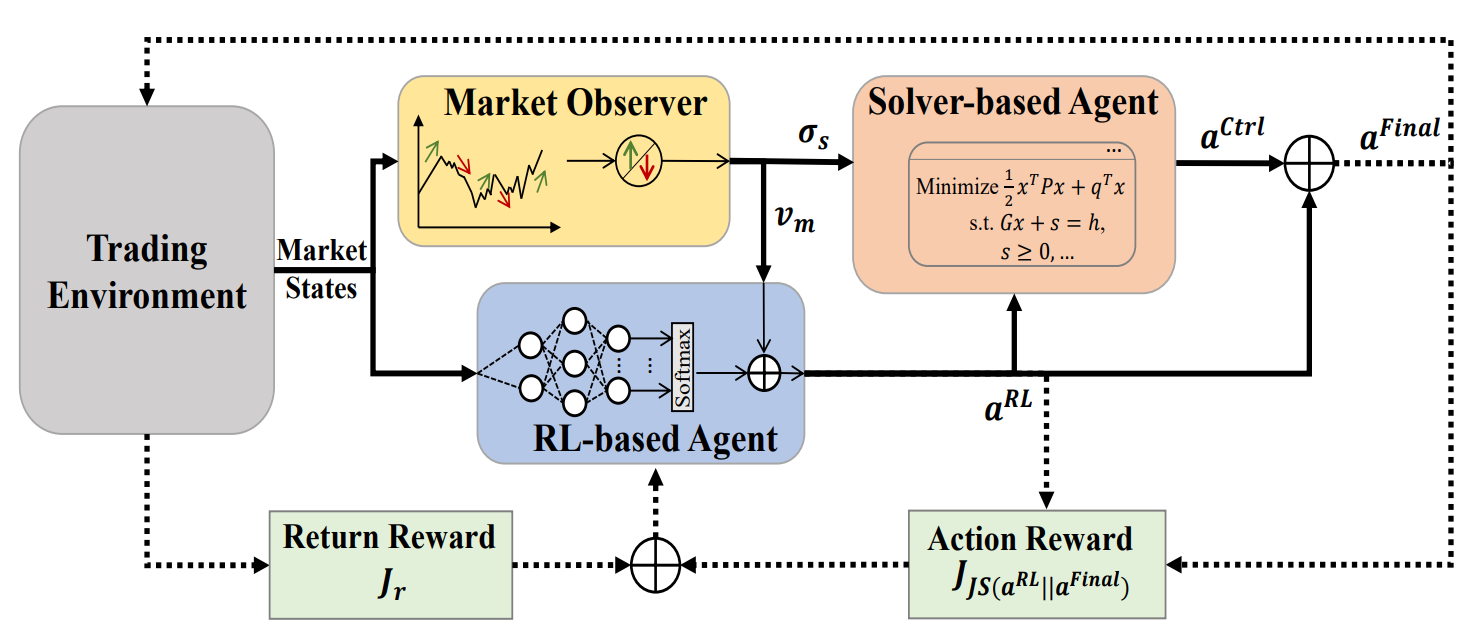
In the previous article, we we introduced the MASA framework — a multi-agent system built on a unique integration of interacting agents. Within the MASA architecture, the RL agent, based on reinforcement learning (RL), optimizes the overall return of an investment portfolio. At the same time, an alternative algorithm-based agent attempts to optimize the portfolio proposed by the RL agent, focusing on minimizing potential risks.

Thanks to a clear division of responsibilities between agents, the model continuously learns and adapts to the underlying financial market environment. The MASA multi-agent scheme achieves more balanced portfolios, both in terms of profitability and in terms of risk exposure.

The original visualization of the MASA framework is provided below.

In the practical section of the previous article, we examined the algorithms implementing the functionality of individual MASA framework agents, developed as separate objects. Today, we continue this work.

1. The MASA Composite Layer

In the previous article, we created three separate agents, each with a specific function within the MASA framework. Now, we will combine them into a single system. For this, we will create a new object CNeuronMASA, whose structure is shown below.

class CNeuronMASA    :  public CNeuronBaseSAMOCL
  {
protected:
   CNeuronMarketObserver   cMarketObserver;
   CNeuronRevINDenormOCL   cRevIN;
   CNeuronRLAgent          cRLAgent;
   CNeuronControlAgent     cControlAgent;
   //---
   virtual bool      feedForward(CNeuronBaseOCL *NeuronOCL) override;
   virtual bool      calcInputGradients(CNeuronBaseOCL *NeuronOCL) override { return false; }
   virtual bool      calcInputGradients(CNeuronBaseOCL *NeuronOCL, CBufferFloat *SecondInput, 
                                                                   CBufferFloat *SecondGradient, 
                                                        ENUM_ACTIVATION SecondActivation = None) override;
   virtual bool      updateInputWeights(CNeuronBaseOCL *NeuronOCL) override;

public:
                     CNeuronMASA(void) {};
                    ~CNeuronMASA(void) {};
   //---
   virtual bool      Init(uint numOutputs, uint myIndex, COpenCLMy *open_cl,
                          uint window, uint window_key, uint units_count,
                          uint heads, uint layers_mo, uint forecast,
                          uint segments_rl, float rho,
                          uint layers_rl, uint n_actions,
                          uint heads_contr,
                          uint layers_contr,
                          int NormLayer, CNeuronBatchNormOCL *normLayer,
                          ENUM_OPTIMIZATION optimization_type, uint batch);
   //---
   virtual int       Type(void) override   const   {  return defNeuronMASA; }
   //---
   virtual bool      Save(int const file_handle) override;
   virtual bool      Load(int const file_handle) override;
   //---
   virtual bool      WeightsUpdate(CNeuronBaseOCL *source, float tau) override;
   virtual void      SetOpenCL(COpenCLMy *obj) override;
   virtual void      SetActivationFunction(ENUM_ACTIVATION value) override;
   //---
   virtual int       GetNormLayer(void)   {  return cRevIN.GetNormLayer(); }
   virtual bool      SetNormLayer(int NormLayer, CNeuronBatchNormOCL *normLayer);
  };

There are several aspects of this new object's structure that deserve special attention.

First, one immediately notices the relatively large number of parameters in the initialization method Init. This is due to the need to accommodate all three agents, each with its own architectural specifics.

Another nuance goes against the general philosophy of our library. The feed-forward pass method has a single input source, which is consistent with the MASA framework. Both the RL agent and the market-observer agent receive the current market state as input. However, in the gradient distribution method, we introduce a second data source - one absent from both the feed-forward pass and the MASA framework as originally described.

This unconventional solution was adopted to enable an alternative training process for the market-observer agent. For this purpose, we also added an internal object for data reverse-normalization. We will discuss this decision in greater detail while building our class methods.

All internal objects of our new class are declared static, allowing us to keep the constructor and destructor empty. Initialization of a new class instance is handled exclusively by the Init method. As mentioned above, this method takes many parameters, though they essentially duplicate the initialization parameters of the previously created agents.

bool CNeuronMASA::Init(uint numOutputs, uint myIndex, COpenCLMy *open_cl,
                       uint window, uint window_key, uint units_count,
                       uint heads_mo, uint layers_mo, uint forecast, uint segments_rl,
                       float rho, uint layers_rl, uint n_actions, uint heads_contr,
                       uint layers_contr, int NormLayer, CNeuronBatchNormOCL *normLayer,
                       ENUM_OPTIMIZATION optimization_type, uint batch)
  {
   if(!CNeuronBaseSAMOCL::Init(numOutputs, myIndex, open_cl, n_actions, rho, optimization_type, batch))
      return false;

Inside the method, we first call the identically named method of the parent class. In this case, the parent class is a fully connected neural layer with SAM optimization.

Recall that the final output of the MASA framework is generated by the controller agent as an action tensor. Accordingly, in the parent class initialization, we set the layer size to match the Actor's action space.

Next, we sequentially initialize our agents. The first is the market-observer agent.

It receives the current market state tensor as input and returns forecast values in the same multimodal sequence format for the specified planning horizon.

//--- Market Observation
   if(!cMarketObserver.Init(0, 0, OpenCL, window, window_key, units_count, heads_mo, layers_mo, forecast,
                                                                                    optimization, iBatch))
      return false;
   if(!cRevIN.Init(0, 1, OpenCL, cMarketObserver.Neurons(), NormLayer, normLayer))
      return false;

Immediately after, we initialize the reverse-normalization layer, whose size matches the output of the market-observer agent.

We then initialize the RL agent, which also receives the market state tensor as input. But it returns the Actor's action tensor in accordance with the learned policy.

//--- RL Agent
   if(!cRLAgent.Init(0, 2, OpenCL, window, units_count, segments_rl, fRho, layers_rl, n_actions, optimization, iBatch))
      return false;

Finally, we initialize the controller agent, which takes the outputs of both previous agents and produces the adjusted Actor action tensor.

   if(!cControlAgent.Init(0, 3, OpenCL, 3, window_key, n_actions / 3, heads_contr, window, forecast, layers_contr,
                                                                                            optimization, iBatch))
      return false;

It is important to note that in our implementation, the RL agent and the controller agent interpret the Actor action tensor differently. The distinction is not merely functional.

The RL agent's output uses a fully connected layer that independently generates each element of the action tensor, based on market analysis and the learned policy. However, we have prior knowledge that opposite actions (buying vs. selling the same asset) are mutually exclusive. Moreover, trade parameters in each direction occupy three elements in the action vector.

Taking this into account, we instruct the controller agent to interpret the action tensor as a multimodal sequence, where each element represents a trade described by a 3-element vector. This way, the controller agent can evaluate risks for each trade direction separately.

At the end of the initialization method, we reassign pointers to external interface buffers and set the sigmoid activation function as default.

   if(!SetOutput(cControlAgent.getOutput(), true) ||
      !SetGradient(cControlAgent.getGradient(), true))
      return false;
   SetActivationFunction(SIGMOID);
//---
   return true;
  }

The method then returns a logical flag indicating successful execution.

A few words should be said on the activation function. The output of our class is the Actor's action tensor - generated first by the RL agent and then adjusted by the controller agent. Obviously, the output spaces must be consistent across both agents and the class itself. For this reason, we override the activation function method to ensure synchronization across all components.

void CNeuronMASA::SetActivationFunction(ENUM_ACTIVATION value)
  {
   cControlAgent.SetActivationFunction(value);
   cRLAgent.SetActivationFunction((ENUM_ACTIVATION)cControlAgent.Activation());
   CNeuronBaseSAMOCL::SetActivationFunction((ENUM_ACTIVATION)cControlAgent.Activation());
  }

After completing initialization, we move on to the feed-forward pass algorithm. This part is straightforward. We simply call the feed-forward methods of our agents in sequence. First, we obtain the market analysis results and the preliminary Actor action tensor.

bool CNeuronMASA::feedForward(CNeuronBaseOCL *NeuronOCL)
  {
   if(!cMarketObserver.FeedForward(NeuronOCL.AsObject()))
      return false;
   if(!cRLAgent.FeedForward(NeuronOCL.AsObject()))
      return false;

Next, we pass these results to the controller agent to produce the final decision.

   if(!cControlAgent.FeedForward(cRLAgent.AsObject(), cMarketObserver.getOutput()))
      return false;
//---
   return true;
  }

The method ends by returning a logical execution result.

Looking again at the earlier visualization of MASA, you might notice that the final action vector is depicted as the sum of the RL agent's and the controller agent's outputs. In our implementation, however, we treat the controller agent's output as the final result, without residual connections to the RL agent. Do you remember the architecture of our controller agent?

Our controller agent is implemented as a Transformer decoder. As you know, the Transformer architecture already includes residual connections in both the attention modules and the FeedForward block. Therefore, residual information flow from the RL agent is inherently built into the controller agent, and additional connections are unnecessary.

We now turn to the backpropagation process. Specifically to the algorithm for error gradient distribution (calcInputGradients). This is where some of our earlier non-standard decisions, which we started in the CNeuronMASA, come into play.

First, let's look at the expected outputs of our agents. Two of our agents return the Actor action tensor. It is logical during training to use the set of optimal actions as the target (in supervised learning) or their projection onto rewards (in reinforcement learning).

However, the market-observer agent outputs forecast values of a multimodal time series for the analyzed financial instrument. This raises the question of training targets for this agent. We could pass gradients through the controller agent to indirectly affect the market-observer's decision to adjust the RL agent output. However, such an approach would not align with its forecasting objective.

A more appropriate solution would be to train the market-observer agent separately on predicting the time series, as we previously did with the Account State Encoder. The challenge, however, is that the observer is now integrated into our composite model. This makes separate training impractical. This brings us to the idea of providing two training targets at the layer level. Which is a fundamental change to our library's workflow. This would require large-scale redesign.

To avoid this, we can adopt a non-standard solution. Let's use the second input source mechanism to deliver an additional set of target values. So, we redefine the error gradient distribution method using two sources of input data, only this time the buffers of the second object will be used to pass the target value tensor to the market observer agent.

bool CNeuronMASA::calcInputGradients(CNeuronBaseOCL *NeuronOCL, CBufferFloat *SecondInput, 
                                                             CBufferFloat *SecondGradient, 
                                                     ENUM_ACTIVATION SecondActivation = -1)
  {
   if(!NeuronOCL)
      return false;

Yet this approach has its pitfalls, primarily data comparability. Usually we feed the model with raw, unprocessed input data received from the terminal. This data from the terminal is normalized in preprocessing, and all neural layers work with normalized values. This also applies to the CNeuronMASA object we are creating. The observer agent's output is therefore also normalized for easier processing by the controller agent. By contrast, the future actual values of the analyzed multimodal time series (our targets) are available only in raw form. To resolve this, we introduced the reverse-normalization layer, which we didn't use in the feed-forward pass. But it is employed during gradient distribution. It re-applies the statistical parameters of the input data to the observer's predictions.

   if(!cRevIN.FeedForward(cMarketObserver.AsObject()))
      return false;

This enables a valid comparison with raw targets and proper gradient propagation.

   if(!cRevIN.FeedForward(cMarketObserver.AsObject()))
      return false;
   float error = 1.0f;
   if(!cRevIN.calcOutputGradients(SecondGradient, error))
      return false;
   if(!cMarketObserver.calcHiddenGradients(cRevIN.AsObject()))
      return false;

Afterward, we distribute the controller agent's gradient between the RL agent and the market-observer. To preserve previously accumulated gradients, we store the observer's error in a buffer, then sum the contributions from both information flows.

   if(!cRLAgent.calcHiddenGradients(cControlAgent.AsObject(), cMarketObserver.getOutput(),
                                    cMarketObserver.getPrevOutput(),
                                    (ENUM_ACTIVATION)cMarketObserver.Activation()) ||
      !SumAndNormilize(cMarketObserver.getGradient(), cMarketObserver.getPrevOutput(), 
                                 cMarketObserver.getGradient(), 1, false, 0, 0, 0, 1))
      return false;

Another key point: both the RL agent and the controller agent return Actor action tensors. The former returns it based on the results of its own analysis of the current market situation. And the latter - after evaluating the risks of the provided action tensor, taking into account the predicted values of the upcoming price movement received from the market observation agent. Ideally, their outputs should coincide. Thus, we introduce an error term for the RL agent representing the deviation from the controller agent's results.

   CBufferFloat *temp = cRLAgent.getGradient();
   if(!cRLAgent.SetGradient(cRLAgent.getPrevOutput(), false) ||
      !cRLAgent.calcOutputGradients(cControlAgent.getOutput(), error) ||
      !SumAndNormilize(temp, cRLAgent.getPrevOutput(), temp, 1, false, 0, 0, 0, 1) ||
      !cRLAgent.SetGradient(temp, false))
      return false;

Once again, these error operations must not erase previously accumulated gradients. To secure this, we use buffer substitution and summation across both data streams.

With gradients distributed among all internal agents, the next step is to pass them back to the input level. Here too, we must aggregate gradients from two sources: the RL agent and the market-observer agent. As before, we first propagate the observer's gradient.

   if(!NeuronOCL.calcHiddenGradients(cMarketObserver.AsObject()))
      return false;

Then we substitute buffers and propagate the RL agent's gradient.

   temp = NeuronOCL.getGradient();
   if(!NeuronOCL.SetGradient(NeuronOCL.getPrevOutput(), false) ||
      !NeuronOCL.calcOutputGradients(cRLAgent.getOutput(), error) ||
      !SumAndNormilize(temp, NeuronOCL.getPrevOutput(), temp, 1, false, 0, 0, 0, 1) ||
      !NeuronOCL.SetGradient(temp, false))
      return false;
//---
   return true;
  }

We sum both contributions and restore the original buffer state.

At this stage, the error gradient has been distributed across all components according to their contribution to the model's performance. The final step is to update model parameters to minimize error. This functionality is performed in the updateInputWeights method. The method algorithm is quite simple. We simply call the feed-forward methods of our agents in sequence. We will not go into detail here. One must only remember that all agents use SAM optimization. Therefore, these updates must be executed in the reverse order of the feed-forward pass.

With this, we conclude our discussion of the algorithms behind the new CNeuronMASA class methods. The full code of this object and all its methods is provided in the attachment for further study.

2. Model Architecture

Now that we have completed the construction of new objects, we move on to the architecture of the trainable models. Here too, we introduced several changes and some unconventional solutions.

First, we abandoned the use of a separate Environment State Encoder. This is no coincidence. In our CNeuronMASA class, two agents already perform parallel analysis of the current environment.

The second modification concerns the inclusion of account state information. Previously, we fed this data into the Actor model as a second input source. Now, however, this input channel is occupied by the target values of the market-observer agent. To resolve this, we simply appended the account state information to the end of the environment state tensor.

Thus, the Actor now receives a combined input tensor consisting of both the environment state description and the account state information.

bool CreateDescriptions(CArrayObj *&actor, CArrayObj *&critic)
  {
//---
   CLayerDescription *descr;
//---
   if(!actor)
     {
      actor = new CArrayObj();
      if(!actor)
         return false;
     }
   if(!critic)
     {
      critic = new CArrayObj();
      if(!critic)
         return false;
     }
//--- Actor
   actor.Clear();
//---
   if(!(descr = new CLayerDescription()))
      return false;
   descr.type = defNeuronBaseOCL;
   int prev_count = descr.count = (HistoryBars * BarDescr + AccountDescr);
   descr.activation = None;
   descr.optimization = ADAM;
   if(!actor.Add(descr))
     {
      delete descr;
      return false;
     }

These raw input data are first processed by a batch normalization layer.

//--- layer 1
   if(!(descr = new CLayerDescription()))
      return false;
   descr.type = defNeuronBatchNormOCL;
   descr.count = prev_count;
   descr.batch = 1e4;
   descr.activation = None;
   descr.optimization = ADAM;
   if(!actor.Add(descr))
     {
      delete descr;
      return false;
     }

At this stage, we must note that the account state vector disrupts the structure of the environment state tensor. Its length may differ from the description size of a single element in the multimodal sequence of the analyzed time series, which is incompatible with the structure of the attention modules we employ. To address this, we convert the input data into matrix form using a trainable embedding layer.

//--- layer 2
   if(!(descr = new CLayerDescription()))
      return false;
   descr.type = defNeuronEmbeddingOCL;
   descr.count = 1;
   descr.window_out = BarDescr;
     {
      int temp[HistoryBars + 1];
      if(ArrayInitialize(temp, BarDescr) < (HistoryBars + 1))
         return false;
      temp[HistoryBars] = AccountDescr;
      if(ArrayCopy(descr.windows, temp) < (HistoryBars + 1))
         return false;
     }
   descr.optimization = ADAM;
   if(!actor.Add(descr))
     {
      delete descr;
      return false;
     }

This layer divides the input vector into fixed-length blocks and projects each block into a subspace of predefined dimensionality, regardless of the block's original size. Each block has its own independently trainable projection matrix.

We know that most of the input tensor consists of homogeneous vectors describing individual environment states (bars), and only the final element (account state) differs. Therefore, we initialize the sequence with fixed-length analysis windows and then adjust only the size of the last element.

Importantly, we set the output size of each embedded sequence element equal to the size of a single bar description. This is a very important thing. This is critical: We could theoretically choose any dimensionality for the embedding output. But the market-observer agent returns forecasts in the original input dimensionality. Therefore, the forecasted multimodal time series must match the target values used during training, which are identical to the raw inputs. The circle closed up.

Using trainable embeddings implicitly provides positional encoding. As we mentioned earlier, each sequence element has its own unique projection matrix. Thus, identical vectors at different positions are projected into different subspace representations, ensuring they remain distinguishable during analysis.

The resulting embeddings are then passed into our MASA framework object. Here, several important details deserve attention.

//--- layer 3
   if(!(descr = new CLayerDescription()))
      return false;
   descr.type = defNeuronMASA;
//--- Windows
     {
      int temp[] = {BarDescr, NForecast, 2 * NActions};    
      if(ArrayCopy(descr.windows, temp) < (int)temp.Size())
         return false;
     }
   descr.window_out = 32;
   descr.count = HistoryBars+1;
//--- Heads
     {
      int temp[] = {4, 4};
      if(ArrayCopy(descr.heads, temp) < (int)temp.Size())
         return false;
     }
//--- Layers
     {
      int temp[] = {3, 3, 3};
      if(ArrayCopy(descr.units, temp) < (int)temp.Size())
         return false;
     }
   descr.window = BarDescr;
   descr.probability = Rho;
   descr.step = 1; // Normalization layer
   descr.batch = 1e4;
   descr.activation = None;
   descr.optimization = ADAM;
   if(!actor.Add(descr))
     {
      delete descr;
      return false;
     }

In the dynamic array descr.windows, we specify the key parameters of the sequences analyzed by the internal agents. Here we sequentially indicate the dimensionality of one input sequence element, the forecasting horizon of the subsequent time series, and the Actor's action space.

Special attention should be paid to the last parameter. In designing the internal agent architecture, we initially described a direct dependency between the environment state and the generated action, excluding stochasticity in the Actor's behavior. However, in practice, we implement a stochastic Actor policy. To achieve this, we double the dimensionality of the MASA framework's output action space. This corresponds to the approach we used earlier in organizing stochastic policy. The resulting action vector is logically divided into two equal parts representing the means and variances of the Actor's action space under the analyzed environment state. For this reason, the activation function of this layer is disabled.

Each attention module we use employs four heads. And each agent contains three encoder/decoder layers.

As noted earlier, the MASA framework's output is passed into the latent state layer of a variational autoencoder, which generates stochastic Actor actions according to the specified distribution.

//--- layer 4
   if(!(descr = new CLayerDescription()))
      return false;
   descr.type = defNeuronVAEOCL;
   descr.count = NActions;
   descr.optimization = ADAM;
   if(!actor.Add(descr))
     {
      delete descr;
      return false;
     }

The resulting action vector is projected into the required range using a convolutional layer followed by a sigmoid activation function.

//--- layer 5
   if(!(descr = new CLayerDescription()))
      return false;
   descr.type = defNeuronConvSAMOCL;
   descr.count = NActions / 3;
   descr.window = 3;
   descr.step = 3;
   descr.window_out = 3;
   descr.activation = SIGMOID;
   descr.optimization = ADAM;
   descr.probability = Rho;
   if(!actor.Add(descr))
     {
      delete descr;
      return false;
     }

At the final model output, we apply a frequency alignment layer to match the model's results with the target values.

//--- layer 6
   if(!(descr = new CLayerDescription()))
      return false;
   descr.type = defNeuronFreDFOCL;
   descr.window = NActions;
   descr.count =  1;
   descr.step = int(false);
   descr.probability = 0.7f;
   descr.activation = None;
   descr.optimization = ADAM;
   if(!actor.Add(descr))
     {
      delete descr;
      return false;
     }

The next step is constructing the Critic architecture. Overall, it remains similar to earlier designs. Though there's one major change: removing the separate Environment State Encoder required us to add an environment analysis block directly to the Critic model. For this, we use the PSformer framework to analyze the current state. Notably, the Critic's input data exclude account state information. In my view, this information has little value for the Critic. Trade outcomes depend primarily on market conditions, not the account state at the time of entry.

One could argue that excessively large or small trade volumes could cause execution errors, resulting in no open position. However, trade volume determination is the Actor's responsibility. Should the Critic handle such edge cases? This is fundamentally a matter of functional separation between the models.

Another consideration is open positions and accumulated profit or loss, i.e., the results of past trades. The Critic evaluates the current trade (or policy), not previous outcomes. Even if we assume the Critic evaluates the policy as a whole, its assessment extends to the end of the episode, not retroactively.

Therefore, the Critic receives only the current environment state as input.

//--- Critic
   critic.Clear();
//--- Input layer
   if(!(descr = new CLayerDescription()))
      return false;
   descr.type = defNeuronBaseOCL;
   prev_count = descr.count = (HistoryBars * BarDescr);
   descr.activation = None;
   descr.optimization = ADAM;
   if(!critic.Add(descr))
     {
      delete descr;
      return false;
     }

As before, the raw input data is processed in a batch normalization layer.

//--- layer 1
   if(!(descr = new CLayerDescription()))
      return false;
   descr.type = defNeuronBatchNormOCL;
   descr.count = prev_count;
   descr.batch = 1e4;
   descr.activation = None;
   descr.optimization = ADAM;
   if(!critic.Add(descr))
     {
      delete descr;
      return false;
     }

Then it is feed onto 3 successive layers of the PSformer framework.

//--- layer 2 - 4
   for(int i = 0; i < 3; i++)
     {
      if(!(descr = new CLayerDescription()))
         return false;
      descr.type = defNeuronPSformer;
      descr.window = BarDescr;
      descr.count = HistoryBars;
      descr.window_out = Segments;
      descr.probability = Rho;
      descr.batch = 1e4;
      descr.activation = None;
      descr.optimization = ADAM;
      if(!critic.Add(descr))
        {
         delete descr;
         return false;
        }
     }

Next, we use successively convolutional and fully connected layers to reduce the dimensionality of the resulting tensor.

//--- layer 5
   if(!(descr = new CLayerDescription()))
      return false;
   descr.type = defNeuronConvSAMOCL;
   descr.count = HistoryBars;
   descr.window = BarDescr;
   descr.step = BarDescr;
   descr.window_out = int(LatentCount / descr.count);
   descr.probability = Rho;
   descr.activation = GELU;
   descr.optimization = ADAM;
   if(!critic.Add(descr))
     {
      delete descr;
      return false;
     }
//--- layer 6
   if(!(descr = new CLayerDescription()))
      return false;
   descr.type = defNeuronBaseSAMOCL;
   descr.count = LatentCount;
   descr.probability = Rho;
   descr.activation = None;
   descr.optimization = ADAM;
   if(!critic.Add(descr))
     {
      delete descr;
      return false;
     }

We combine the results of the environmental analysis with the agent's actions in the data concatenation layer.

//--- layer 7
   if(!(descr = new CLayerDescription()))
      return false;
   descr.type = defNeuronConcatenate;
   descr.count = LatentCount;
   descr.window = LatentCount;
   descr.step = NActions;
   descr.activation = GELU;
   descr.optimization = ADAM;
   if(!critic.Add(descr))
     {
      delete descr;
      return false;
     }

After that comes the decision-making module, which consists of 4 fully connected layers.

//--- layer 8
   if(!(descr = new CLayerDescription()))
      return false;
   descr.type = defNeuronBaseSAMOCL;
   descr.count = LatentCount;
   descr.activation = SIGMOID;
   descr.optimization = ADAM;
   descr.probability = Rho;
   if(!critic.Add(descr))
     {
      delete descr;
      return false;
     }
//--- layer 9
   if(!(descr = new CLayerDescription()))
      return false;
   descr.type = defNeuronBaseSAMOCL;
   descr.count = LatentCount;
   descr.activation = SIGMOID;
   descr.optimization = ADAM;
   descr.probability = Rho;
   if(!critic.Add(descr))
     {
      delete descr;
      return false;
     }
//--- layer 10
   if(!(descr = new CLayerDescription()))
      return false;
   descr.type = defNeuronBaseSAMOCL;
   descr.count = LatentCount;
   descr.activation = SIGMOID;
   descr.optimization = ADAM;
   descr.probability = Rho;
   if(!critic.Add(descr))
     {
      delete descr;
      return false;
     }
//--- layer 11
   if(!(descr = new CLayerDescription()))
      return false;
   descr.type = defNeuronBaseSAMOCL;
   descr.count = NRewards;
   descr.activation = None;
   descr.optimization = ADAM;
   descr.probability = Rho;
   if(!critic.Add(descr))
     {
      delete descr;
      return false;
     }

At the output stage, we use a frequency alignment layer to reconcile the model's results with the target values.

//--- layer 12
   if(!(descr = new CLayerDescription()))
      return false;
   descr.type = defNeuronFreDFOCL;
   descr.window = NRewards;
   descr.count =  1;
   descr.step = int(false);
   descr.probability = 0.7f;
   descr.activation = None;
   descr.optimization = ADAM;
   if(!critic.Add(descr))
     {
      delete descr;
      return false;
     }
//---
   return true;
  }

After successfully defining the architectures of the two trainable models, we complete the method by returning a logical result to the calling program.

3. Model Training Program

We are now confidently approaching the logical conclusion of our work and turn to the construction of the model training program. Naturally, removing one of the trainable models has left its mark on the training algorithm. Moreover, when designing the MASA framework module, we agreed to use the information stream from the second data source as an additional flow of target values. With that in mind, let us proceed directly to the training algorithm, implemented in the Train method.

As before, we begin with some preparatory work. We form a vector of trajectory selection probabilities from the experience replay buffer, weighted by the effectiveness of past runs.

void Train(void)
  {
//---
   vector<float> probability = GetProbTrajectories(Buffer, 0.9);
//---
   vector<float> result, target, state;
   bool Stop = false;
//---
   uint ticks = GetTickCount();

We then declare the necessary local variables.

Next, we set up the training loop, where the number of iterations is determined by the external parameters of our Expert Advisor.

   for(int iter = 0; (iter < Iterations && !IsStopped() && !Stop); iter ++)
     {
      int tr = SampleTrajectory(probability);
      int i = (int)((MathRand() * MathRand() / MathPow(32767, 2)) * (Buffer[tr].Total - 2 - NForecast));
      if(i <= 0)
        {
         iter --;
         continue;
        }
      if(!state.Assign(Buffer[tr].States[i].state) ||
         MathAbs(state).Sum() == 0 ||
         !bState.AssignArray(state))
        {
         iter --;
         continue;
        }
      if(!state.Assign(Buffer[tr].States[i+NForecast].state) ||
         !state.Resize(NForecast*BarDescr) ||
         MathAbs(state).Sum() == 0 ||
         !bForecast.AssignArray(state))
        {
         iter --;
         continue;
        }

Within the loop, we sample one trajectory and its environment state. At this point, we also verify the presence of both historical and future data at the required analysis depth and forecasting horizon. If the check fails at any point, we resample a new trajectory and state.

Once the necessary data are available, we transfer them into the appropriate buffers. We then append account state information to the environment state description at the time of analysis.

      //--- Account
      float PrevBalance = Buffer[tr].States[MathMax(i - 1, 0)].account[0];
      float PrevEquity = Buffer[tr].States[MathMax(i - 1, 0)].account[1];
      bState.Add((Buffer[tr].States[i].account[0] - PrevBalance) / PrevBalance);
      bState.Add(Buffer[tr].States[i].account[1] / PrevBalance);
      bState.Add((Buffer[tr].States[i].account[1] - PrevEquity) / PrevEquity);
      bState.Add(Buffer[tr].States[i].account[2]);
      bState.Add(Buffer[tr].States[i].account[3]);
      bState.Add(Buffer[tr].States[i].account[4] / PrevBalance);
      bState.Add(Buffer[tr].States[i].account[5] / PrevBalance);
      bState.Add(Buffer[tr].States[i].account[6] / PrevBalance);

We also add a timestamp to the analyzed environment state.

      //---
      double time = (double)Buffer[tr].States[i].account[7];
      double x = time / (double)(D'2024.01.01' - D'2023.01.01');
      bState.Add((float)MathSin(x != 0 ? 2.0 * M_PI * x : 0));
      x = time / (double)PeriodSeconds(PERIOD_MN1);
      bState.Add((float)MathCos(x != 0 ? 2.0 * M_PI * x : 0));
      x = time / (double)PeriodSeconds(PERIOD_W1);
      bState.Add((float)MathSin(x != 0 ? 2.0 * M_PI * x : 0));
      x = time / (double)PeriodSeconds(PERIOD_D1);
      bState.Add((float)MathSin(x != 0 ? 2.0 * M_PI * x : 0));

After preparing the input data, we begin the model training process. The first step is training the Critic. The Critic receives as input the analyzed environment state and the action vector actually performed by the Actor when the training sample was collected. We use these actions because we already know the real rewards provided by the environment for them. We perform a feed-forward pass, evaluating the Actor's past actions.

      //--- Critic
      bActions.AssignArray(Buffer[tr].States[i].action);
      Critic.TrainMode(true);
      if(!Critic.feedForward((CBufferFloat*)GetPointer(bState), 1, false, (CBufferFloat*)GetPointer(bActions)))
        {
         PrintFormat("%s -> %d", __FUNCTION__, __LINE__);
         Stop = true;
         break;
        }

As expected, we want the Critic's feed-forward pass output to be a reward tensor close to the actual rewards observed. Therefore, we extract the factual reward from the replay buffer and run the Critic's backpropagation process, minimizing error against this target.

      result.Assign(Buffer[tr].States[i + 1].rewards);
      target.Assign(Buffer[tr].States[i + 2].rewards);
      result = result - target * DiscFactor;
      Result.AssignArray(result);
      if(!Critic.backProp(Result, (CBufferFloat *)GetPointer(bActions), (CBufferFloat *)GetPointer(bGradient)))
        {
         PrintFormat("%s -> %d", __FUNCTION__, __LINE__);
         Stop = true;
         break;
        }

Next comes Actor policy training, which we conduct in two stages. First, the Actor performs a forward pass to generate an action tensor.

      //--- Actor Policy
      if(!Actor.feedForward((CBufferFloat*)GetPointer(bState), 1, false, (CBufferFloat*)NULL))
        {
         PrintFormat("%s -> %d", __FUNCTION__, __LINE__);
         Stop = true;
         break;
        }

This is followed by a feed-forward pass of the Critic, this time evaluating the Actor's generated actions.

      Critic.TrainMode(false);
      if(!Critic.feedForward((CBufferFloat*)GetPointer(bState), 1, false, (CNet*)GetPointer(Actor), LatentLayer))
        {
         PrintFormat("%s -> %d", __FUNCTION__, __LINE__);
         Stop = true;
         break;
        }

At this stage, Critic training is disabled. This will prevent incorrect values from influencing the Actor's reward policy learning.

We then evaluate the outcome of the analyzed trajectory. If the Actor’s policy produced a positive result, we shift the Actor's current policy toward that positive trajectory in a supervised learning style. This constitutes the first stage of Actor training.

      if(Buffer[tr].States[0].rewards[0] > 0)
         if(!Actor.backProp(GetPointer(bActions),(CBufferFloat*)GetPointer(bForecast),GetPointer(bGradient)))
           {
            PrintFormat("%s -> %d", __FUNCTION__, __LINE__);
            Stop = true;
            break;
           }

In the second stage, we assign the Critic the task of maximizing reward and propagate the error gradient down to the Actor's action level.

      Critic.getResults(Result);
      for(int c = 0; c < Result.Total(); c++)
        {
         float value = Result.At(c);
         if(value >= 0)
            Result.Update(c, value * 1.01f);
         else
            Result.Update(c, value * 0.99f);
        }
      if(!Critic.backProp(Result, (CNet *)GetPointer(Actor), LatentLayer) ||
         !Actor.backPropGradient((CBufferFloat*)GetPointer(bForecast),GetPointer(bGradient)))
        {
         PrintFormat("%s -> %d", __FUNCTION__, __LINE__);
         Stop = true;
         break;
        }

This enables the Critic to indicate the direction in which the Actor's policy should be adjusted to increase overall returns. The Actor's policy is then updated accordingly.

We continue to inform the user about the training process and proceed to the next iteration of the training cycle.

      //---
      if(GetTickCount() - ticks > 500)
        {
         double percent = double(iter) * 100.0 / (Iterations);
         string str = StringFormat("%-14s %6.2f%% -> Error %15.8f\n", "Actor", percent, Actor.getRecentAverageError());
         str += StringFormat("%-14s %6.2f%% -> Error %15.8f\n", "Critic", percent, Critic.getRecentAverageError());
         Comment(str);
         ticks = GetTickCount();
        }
     }

After successfully completing all iterations, we clear the comments field on the instrument chart (used to display user information).

   Comment("");
//---
   PrintFormat("%s -> %d -> %-15s %10.7f", __FUNCTION__, __LINE__, "Actor", Actor.getRecentAverageError());
   PrintFormat("%s -> %d -> %-15s %10.7f", __FUNCTION__, __LINE__, "Critic", Critic.getRecentAverageError());
   ExpertRemove();
//---
  }

Output the model training results to the log and initiate the EA termination process.

At this point, we conclude our discussion of the MASA framework algorithms and the implementation of model training programs. The full source code is available in the attachment.

4. Testing

So, our work on implementing the approaches proposed by the authors of the MASA framework using MQL5 has come to its logical conclusion. We have now reached the final stage of our work – the evaluation of the implemented approaches on real historical data.

It is important to emphasize that we are assessing the effectiveness of the implemented approaches, not merely the proposed ones, as our implementation included several modifications to the original MASA framework.

The models were trained on EURUSD H1 data from 2023. All indicator parameters were set to their default values.

For initial training, we used a dataset compiled in earlier work, periodically updated throughout training to keep it aligned with the Actor's evolving policy.

After several cycles of model training and dataset updates, we obtained a policy that demonstrated profitability on both the training and testing sets.

The trained policy was tested on historical data from January 2024, with all other parameters unchanged. The results are as follows:

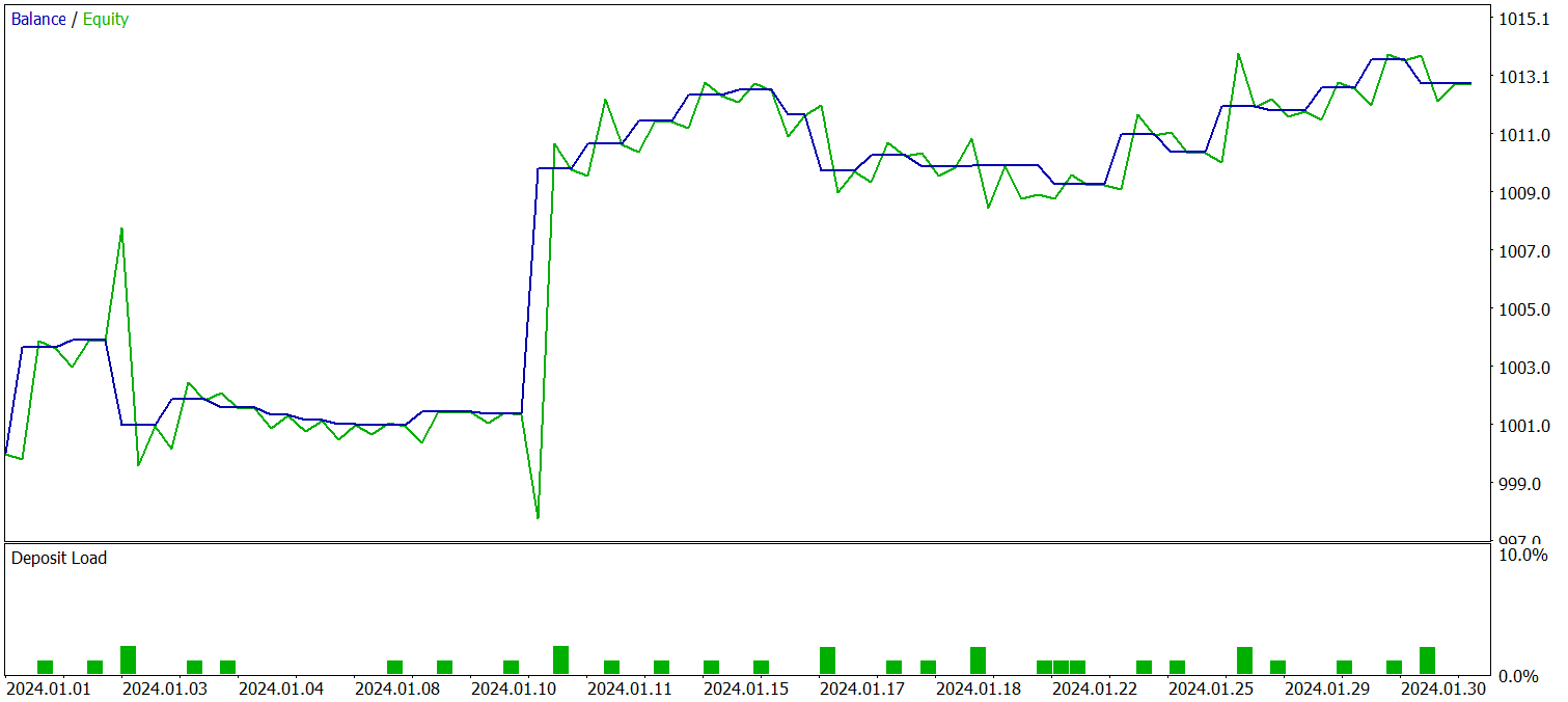
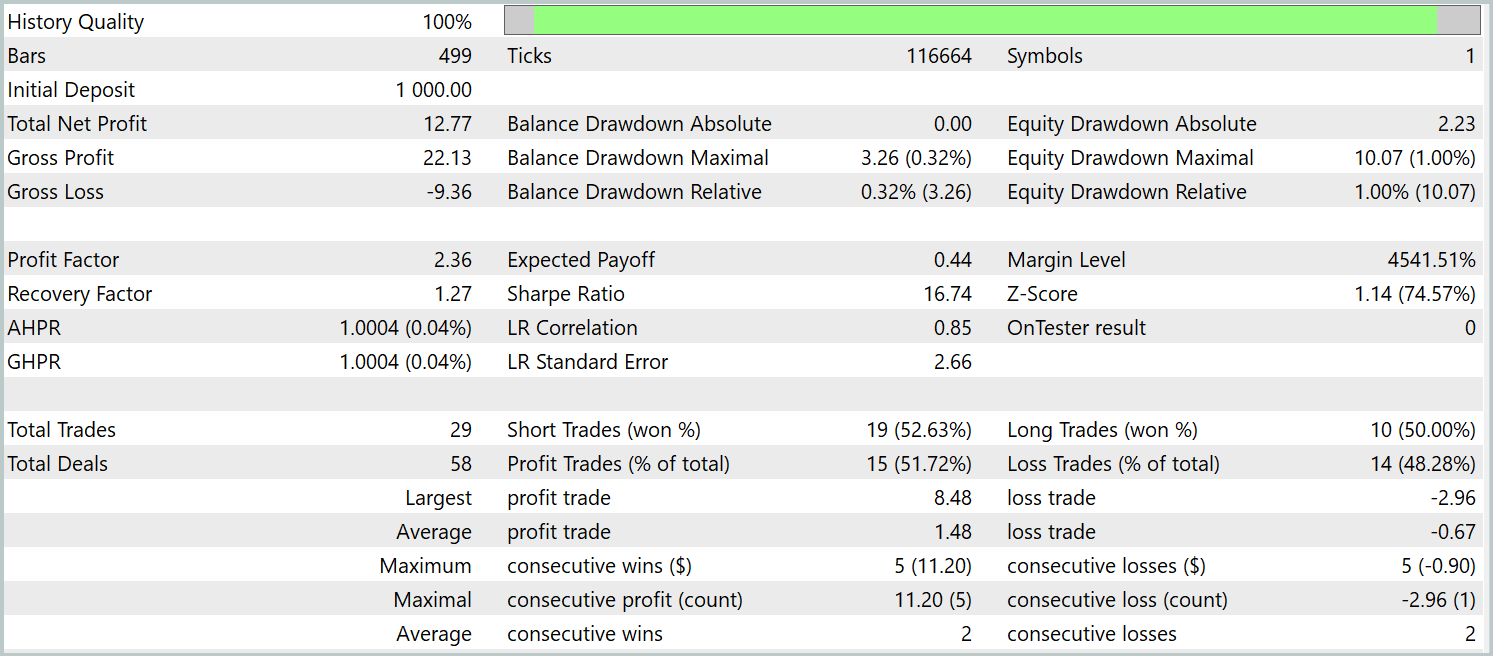
During the test period, the model executed 29 trades, half of which closed with profit. Thanks to the fact that the average profitable trade was more than twice the size of the average losing trade, the model achieved a clear upward trend in account balance. These results point to the potential of the implemented framework. 

Conclusion

We have explored an innovative methodology for portfolio management in unstable financial markets – the MASA multi-agent adaptive system. This framework effectively combines the strengths of RL algorithms and adaptive optimization methods, enabling models to simultaneously improve profitability and reduce risk.

In the practical section, we implemented our interpretation of the proposed approaches in MQL5. We trained models on real historical data, and tested the resulting policies. The results indicate promising potential. Nevertheless, before deployment in live trading, it is essential to conduct further training on more representative datasets and perform extensive testing under a variety of conditions.

References

• Developing A Multi-Agent and Self-Adaptive Framework with Deep Reinforcement Learning for Dynamic Portfolio Risk Management
• Other articles from this series

Programs used in the article

#	Name	Type	Description
1	Research.mq5	Expert Advisor	Expert Advisor for collecting examples
2	ResearchRealORL.mq5	Expert Advisor	Expert Advisor for collecting examples using the Real-ORL method
3	Study.mq5	Expert Advisor	Model training Expert Advisor
4	Test.mq5	Expert Advisor	Model testing Expert Advisor
5	Trajectory.mqh	Class library	System state description structure
6	NeuroNet.mqh	Class library	A library of classes for creating a neural network
7	NeuroNet.cl	Library	OpenCL program code library