Overcoming The Limitation of Machine Learning (Part 3): A Fresh Perspective on Irreducible Error

This article will introduce the reader to advanced limitations of current machine learning models that are not explicitly taught to instructors before they deploy these models. The field of machine learning is dominated by mathematical notation and literature. And since there are many levels of abstraction from which a practitioner can study, the approach often differs. For example, some practitioners study machine learning simply from high-level libraries such as scikit-learn, which provide an easy and intuitive framework to use models while abstracting away the mathematical concepts that underpin them.

However, depending on the level of mastery and the amount of control the practitioner desires, sometimes these abstractions must be removed to see what’s really going on under the hood. Therefore, in any project involving machine learning models, irreducible error is always present, though it is rarely mentioned directly.

Let us consider the formula for simple linear regression. Normally, the target we are trying to predict, Y, can be thought of as a function, f, of some inputs we can measure, X, that are transformed by a set of coefficients, B, to produce the target, Y, given some amount of random noise we cannot observe or control, e. Our discussion today is focused on this error term, e, that silently lives in all machine learning models. Our objective is to show the reader that this error term is not entirely as random as classical literature would lead us to believe. Believing that this error term is random and totally irreducible appears contrary to the truth.

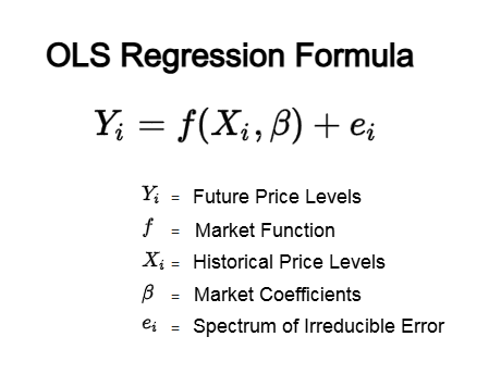
Figure 1: Mathematical explanations of ordinary least squares regression give few details on the irreducible error terms and what caused them

Our sole objective is to give the reader a fresh perspective on irreducible error by showing that what is commonly referred to as a single quantity, “irreducible error,” may potentially be decomposed into a spectrum of independent sources of error. The first two are well-established in the scientific community:

1. The inherent variability or natural randomness of the true underlying process.
   
2. The bias of the model itself.

Therefore, our discussion today aims to introduce a third, lesser-known component of irreducible error. The key takeaway of this point is that we can exercise control over this third source of error to improve our trading performance.

Machine learning models can be studied from multiple perspectives, making it difficult for any reader to fully master them all. We often learn about these models from a statistical perspective. However, few readers ever explore them from a geometric perspective—and it is here that the third source of irreducible error lives and hides, out of sight for practitioners who remain at higher levels of abstraction.

This third type of error is not only difficult to fix—hence the term “irreducible”—but also difficult to even notice in the first place. It is often hidden behind terse mathematical notation, which can make it equally difficult for any one of us to see.

Our article makes no claim to reduce this error to zero. Rather, it shows how to use machine learning models more intelligently and appropriately once we recognize that this error exists.

When studied from a geometric perspective, the reader should understand that machine learning models do not truly “learn” the function that maps inputs to outputs. As a matter of fact, the model makes no true attempt at ever directly approximating the function generating the target. 

Think of a human artist drawing an image on paper. The paper acts as the canvas that the artist uses to capture an image of his muse. Similarly, machine learning models use the inputs we provide to create a new "canvas" called a manifold. Now, imagine we held a coin so that it would cast a shadow on the "canvas" our machine learning model created from the inputs we gave it. The point where the shadow strikes the canvas, is the prediction our model makes. But our true target is the true coin. The point intended for the reader to understand is that, our machine learning models are essentially embedding images of the target onto some combination/manifold of the inputs it was given.

But the target you are trying to predict does not necessarily live in the manifold we can create from the inputs —it lives in its own manifold space. Therefore, there is always some irreducible distance between the manifold created by your inputs and the manifold where the true target lives. This is one source of error. Add to it the natural randomness of the process (the second source) and the bias of the model (the third source), and you get the complete picture.

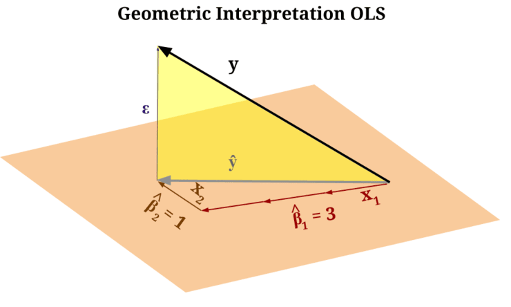
Figure 2: The "orange plane" represents the "canvas" the model created from the inputs you gave it, while the "yellow triangle" is the irreducible error between the canvas and the true target

Readers already familiar with analytical geometry will recognize that the span of the inputs given to a machine learning model defines a new coordinate system. The model then attempts to describe the target using this new coordinate system it learned from the input data. But remember: the target lives in its own coordinate system, independent of the one defined by the inputs!

Advanced readers already familiar with this geometric perspective of machine learning may find the following discussion self-evident, and may consider skimming ahead if they choose to stay with us. For those who have not yet encountered the problem in this way, the remainder of the article is dedicated for you.

The key takeaway is that we can exercise a degree of control over this error in our trading activities by making more conscious, deliberate, and intelligent use of machine learning models.

Our conversation begins with the baseline performance level established in our previous discussion on feedback controllers, the link to which is provided, here. Our feedback controller significantly improved performance compared to where we started in that conversation. After making the adjustments suggested in this article, we subsequently outperformed the old feedback controller, which was already close to acceptable.

Our methodology involved letting go of direct point-to-point comparisons. Instead of asking the model to predict a future price level and comparing it to the current price, we modeled price levels over two time intervals and traded the anticipated slope/trend. In other words, we traded the slope predicted by the model over two intervals, rather than making a direct comparison of predicted and actual prices.

We performed a five-year backtest on the EUR/USD pair using identical strategies, with the only difference being how we instructed our models to model price. The results showed growth in the following dimensions of performance:

Trading Profitability
Our total net profit increased from $245 to $253, a 3% improvement in profitability, while at the same time our Sharpe ratio rose from 0.68 to 0.84, a 23% improvement in Sharpe ratio is remarkable when trading a financial market as challenging as the EUR/USD pair.

Trading Risk
Even more astonishing, was that the gross loss over the 5 year backtest fell from $838 to $721; this represents a 13% reduction in total risk taken on by our trading application. Additionally, our cumulative trading activity fell from 152 trades to 139 trades, an 8% reduction in the total number of trades required. Meaning our application realized larger profit margins while taking on less risk.

Trading Accuracy

Lastly, the proportion of profitable trades rose by 4%, from 57.24% in the original benchmark of our feedback controller, to 59.71% after making the adjustments we suggested.  Meaning that overall, our system became more profitable while taking on less risk—an ideal feature for any trading application.

These modifications should strongly be considered by all practitioners. But let us first start by reviewing the old performance levels established by the first feedback controller we implemented using in our previous discussion.

The first backtest was established from 01 January 2020 until 01 May 2025. We will keep these dates the same even during this second test.

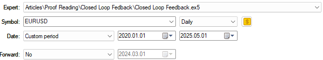
Figure 3: Revisiting the baseline performance levels we established in our opening discussion

The old feedback controller produced results that are truly acceptable, but we can still perform better than this. We have kept these old results here so that the reader can contrast the new results we are about to produce; therefore, Figure 4 below has been taken from our old feedback controller. It serves as a benchmark for us to outperform today.

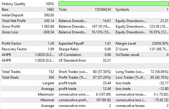
Figure 4: The old performance levels established by our initial attempt to build a feedback controller

The equity curve produced by our old feedback controller was promising. We managed to realize more profit from the strategy by making a few adjustments to the original strategy, that ended up having a pronounced effect on the profitability of our system entirely. In Figure 5 below, we can see that the old feedback controller only managed to rise to the $700 profit level in 2023. However, as we shall soon see, our revised feedback controller reached the $700 profit level in 2021. Albeit, it experienced a shock in profitability shortly after 2021, but needless to say, the improvements made are evident.

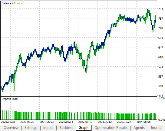
Figure 5: The profit and equity curve produced by the benchmark version of our trading strategy

Getting Started in MQL5

As with all our trading applications, we begin by defining important system definitions carried over from the initial version of our trading strategy, without any changes. Recall that these definitions are important because they help us keep our tests fair and our comparisons consistent.

//+------------------------------------------------------------------+
//|                                     Closed Loop Feedback 1.2.mq5 |
//|                                               Gamuchirai Ndawana |
//|                    https://www.mql5.com/en/users/gamuchiraindawa |
//+------------------------------------------------------------------+
#property copyright "Gamuchirai Ndawana"
#property link      "https://www.mql5.com/en/users/gamuchiraindawa"
#property version   "1.00"

//+------------------------------------------------------------------+
//| System definitions                                               |
//+------------------------------------------------------------------+
#define MA_PERIOD    10
#define FEATURES     12
#define TARGETS      15
#define HORIZON      10
#define OBSERVATIONS 90
#define ACCOUNT_STATES 3

Next, we define important global variables that will be used in the trading strategy. These variables keep track of technical indicators, the condition and state of our trading account, the width of our stop loss, and whether the strategy should trade without making a prediction or make a prediction first before trading. Global variables allow us to define and control the behavior of our application in a way that is both predictable and repeatable.

//+------------------------------------------------------------------+
//| Global variables                                                 |
//+------------------------------------------------------------------+
int    ma_h_handler,ma_l_handler,atr_handler,scenes,b_matrix_scenes;
double ma_h[],ma_l[],atr[];
double padding;
matrix snapshots,OB_SIGMA,OB_VT,OB_U,b_vector,b_matrix;
vector S,prediction;
vector account_state;
bool predict,permission;

All trading applications also have dependencies that help avoid rewriting the same boilerplate code. Therefore, we load important libraries such as the trade library (to open and close positions), along with two custom libraries built for these discussions: the time library and the trade information library. The time library helps us determine when a new candle has formed, while the trade information library provides important details such as the minimum lot size allowed and the current bid and ask prices.

//+------------------------------------------------------------------+
//| Dependencies                                                     |
//+------------------------------------------------------------------+
#include <Trade\Trade.mqh>
#include <VolatilityDoctor\Time\Time.mqh>
#include <VolatilityDoctor\Trade\TradeInfo.mqh>

CTrade      Trade;

Time        *DailyTimeHandler;
TradeInfo   *TradeInfoHandler;

Upon initialization, we create new instances of all the custom classes we’ve built so far. We also define technical indicator instances, such as the moving average and the ATR indicators, as well as the important matrices and vectors we will need. Boolean flags are initialized, and the counter for elapsed scenes is reset to zero each time the application is started. 

//+------------------------------------------------------------------+
//| Expert initialization function                                   |
//+------------------------------------------------------------------+
int OnInit()
  {
//---
   DailyTimeHandler  = new Time(Symbol(),PERIOD_D1);
   TradeInfoHandler  = new TradeInfo(Symbol(),PERIOD_D1);
   ma_h_handler      = iMA(Symbol(),PERIOD_D1,MA_PERIOD,0,MODE_EMA,PRICE_HIGH);
   ma_l_handler      = iMA(Symbol(),PERIOD_D1,MA_PERIOD,0,MODE_EMA,PRICE_LOW);
   atr_handler       = iATR(Symbol(),PERIOD_D1,14);
   snapshots         = matrix::Ones(FEATURES,OBSERVATIONS);
   scenes            = 0;
   b_matrix_scenes   = 0;
   account_state     = vector::Zeros(3);
   b_matrix          = matrix::Zeros(1,1);
   prediction        = vector::Zeros(2);
   predict           = false;
   permission        = true;
//---
   return(INIT_SUCCEEDED);
  }

When the application is no longer in use, it is good practice in MQL5 to practice proper memory management. Therefore, we delete custom object instances and release any technical indicators no longer in use.

//+------------------------------------------------------------------+
//| Expert deinitialization function                                 |
//+------------------------------------------------------------------+
void OnDeinit(const int reason)
  {
//---
   delete DailyTimeHandler;
   delete TradeInfoHandler;
   IndicatorRelease(ma_h_handler);
   IndicatorRelease(ma_l_handler);
   IndicatorRelease(atr_handler);
  }

When new price levels are received from the trade server, our Expert Advisor will also call its OnTick function. In this setup, the first check is whether a new candle has formed. This ensures our backtests run faster, as actions are only performed once per candle.

Once confirmed, we update the technical indicator readings and our pageant variable, which tells us how wide our stop loss should be. We then keep track of the most recent closed price. If there are one or more open positions, we select the tickets of the open positions and modify their stop losses so that they trail as profitability increases.

To set up a trailing stop, we first capture the current values of the stop loss and take profit. By comparing these values to the suggested updated values, we decide whether to update. If the suggested value is more profitable, the update is made; otherwise, no change is applied. Importantly, before performing this update, we must confirm what type of position we are modifying.

If no positions are open, we initialize the account state vector. Recall that this vector keeps track of what type of position we intend to open. If the close price is above the high moving average, we open a buy. If it is below the low moving average, we open a sell.

Trades are opened directly if the predict Boolean flag is set to false and the permission Boolean flag is true. Otherwise, the system records all variables and makes a prediction before opening trades.

//+------------------------------------------------------------------+
//| Expert tick function                                             |
//+------------------------------------------------------------------+
void OnTick()
  {
//---
   if(DailyTimeHandler.NewCandle())
     {
      CopyBuffer(ma_h_handler,0,0,1,ma_h);
      CopyBuffer(ma_l_handler,0,0,1,ma_l);
      CopyBuffer(atr_handler,0,0,1,atr);
      padding = atr[0]*2;
      double c = iClose(Symbol(),PERIOD_D1,0);

      if(PositionsTotal() > 0)
        {
         ulong ticket = PositionSelectByTicket(PositionGetTicket(0));
         if(ticket)
           {
            double sl,tp;

            sl = PositionGetDouble(POSITION_SL);
            tp = PositionGetDouble(POSITION_TP);

            if(PositionGetInteger(POSITION_TYPE) == POSITION_TYPE_BUY)
              {
               double new_sl = TradeInfoHandler.GetBid()-padding;
               double new_tp = TradeInfoHandler.GetBid()+padding;

               if(new_sl > sl)
                  Trade.PositionModify(ticket,new_sl,new_tp);
              }

            else
               if(PositionGetInteger(POSITION_TYPE) == POSITION_TYPE_SELL)
                 {
                  double new_sl = TradeInfoHandler.GetAsk()+padding;
                  double new_tp = TradeInfoHandler.GetAsk()-padding;

                  if(new_sl < sl)
                     Trade.PositionModify(ticket,new_sl,new_tp);
                 }
           }
        }

      if(PositionsTotal() == 0)
        {
         account_state = vector::Zeros(ACCOUNT_STATES);

         if(c > ma_h[0])
           {
            if(!predict)
              {
               if(permission)
                  Trade.Buy(TradeInfoHandler.MinVolume(),Symbol(),TradeInfoHandler.GetAsk(),(TradeInfoHandler.GetBid()-(padding)),(TradeInfoHandler.GetBid()+(padding)),"");
              }

            account_state[0] = 1;
           }

         else
            if(c < ma_l[0])
              {
               if(!predict)
                 {
                  if(permission)
                     Trade.Sell(TradeInfoHandler.MinVolume(),Symbol(),TradeInfoHandler.GetBid(),(TradeInfoHandler.GetAsk()+(padding)),(TradeInfoHandler.GetAsk()-(padding)),"");
                 }

               account_state[1] = 1;
              }

            else
              {
               account_state[2] = 1;
              }
        }

      if(scenes < OBSERVATIONS)
        {
         take_snapshots();
        }

      else
        {
         matrix temp;
         temp.Assign(snapshots);
         snapshots = matrix::Ones(FEATURES,scenes+1);

         //--- The first row is the intercept and must be full of ones
         for(int i=0;i<FEATURES;i++)
            snapshots.Row(temp.Row(i),i);

         take_snapshots();
         fit_snapshots();

         predict = true;
         permission = false;
        }
      scenes++;
     }
  }

The method we use to take a snapshot is straightforward. It records important market information into a matrix we call snapshot. This includes the open, high, low, and close prices, as well as the equity in the account. Readers who have followed earlier discussions will recognize this code, since it is the same as what we used at the beginning of the series.

//+------------------------------------------------------------------+
//| Record the current state of our system                           |
//+------------------------------------------------------------------+
void take_snapshots(void)
  {
   snapshots[1,scenes] = iOpen(Symbol(),PERIOD_D1,1);
   snapshots[2,scenes] = iHigh(Symbol(),PERIOD_D1,1);
   snapshots[3,scenes] = iLow(Symbol(),PERIOD_D1,1);
   snapshots[4,scenes] = iClose(Symbol(),PERIOD_D1,1);
   snapshots[5,scenes] = AccountInfoDouble(ACCOUNT_BALANCE);
   snapshots[6,scenes] = AccountInfoDouble(ACCOUNT_EQUITY);
   snapshots[7,scenes] = ma_h[0];
   snapshots[8,scenes] = ma_l[0];
   snapshots[9,scenes] = account_state[0];
   snapshots[10,scenes] = account_state[1];
   snapshots[11,scenes] = account_state[2];
  }

Now, however, we start to see the improvements made over that initial version. Up to this point, everything should be familiar to returning readers. We are now preparing the inputs and outputs of the system that models how our snapshots evolve. Recall that snapshots track important details of how our strategy interacts with the market—for example, how our account balance and equity change over time.

The X matrix stores the input data, while the Y matrix stores the output data. If the reader looks carefully at the Y matrix, they will notice that rows 4, 5, 6, and 7 of Y are copied from rows 5, 6, 7, and 8 of X. Then, those same rows from X are duplicated again, but shifted into the future. This means we ask our model not only to predict the account balance one step into the future, but also ten steps into the future.

Depending on the trend predicted across these two horizons, we decide whether to open a trade. Once the optimal solution is found using the pseudo-inverse method (discussed previously), our model will output two predictions:

1. The expected balance at the next candle (prediction 4).
   
2. The expected balance after ten candles (prediction 8).

The model then makes trading decisions based on these predictions. If it expects account growth, trades are allowed. If it expects decline, permission is withheld.

This is a significant improvement over the previous method. In earlier discussions, we compared the model’s predicted account balance directly against the current real balance, as if the two were the same. In this approach, we avoid making that mistake.

//+------------------------------------------------------------------+
//| Fit our linear model to our collected snapshots                  |
//+------------------------------------------------------------------+
void fit_snapshots(void)
  {
   matrix X,y;
   X.Reshape(FEATURES,scenes);
   y.Reshape(TARGETS,scenes);

   for(int i=0;i<scenes-HORIZON;i++)
     {
      X[0,i] = snapshots[0,i];
      X[1,i] = snapshots[1,i];
      X[2,i] = snapshots[2,i];
      X[3,i] = snapshots[3,i];
      X[4,i] = snapshots[4,i];
      X[5,i] = snapshots[5,i];
      X[6,i] = snapshots[6,i];
      X[7,i] = snapshots[7,i];
      X[8,i] = snapshots[8,i];
      X[9,i] = snapshots[9,i];
      X[10,i] = snapshots[10,i];
      X[11,i] = snapshots[11,i];

      y[0,i] = snapshots[1,i+1];
      y[1,i] = snapshots[2,i+1];
      y[2,i] = snapshots[3,i+1];
      y[3,i] = snapshots[4,i+1];
      y[4,i] = snapshots[5,i+1];
      y[5,i] = snapshots[6,i+1];
      y[6,i] = snapshots[7,i+1];
      y[7,i] = snapshots[8,i+1];
      y[8,i] = snapshots[5,i+HORIZON];
      y[9,i] = snapshots[6,i+HORIZON];
      y[10,i] = snapshots[7,i+HORIZON];
      y[11,i] = snapshots[8,i+HORIZON];
      y[12,i] = snapshots[9,i+1];
      y[13,i] = snapshots[10,i+1];
      y[14,i] = snapshots[11,i+1];
     }

   if(PositionsTotal() == 0)
     {
      //--- Find optimal solutions
      b_vector = y.MatMul(X.PInv());
      Print("Day Number: ",scenes+1);
      Print("Snapshot");
      Print(snapshots);
      Print("Input");
      Print(X);
      Print("Target");
      Print(y);
      Print("Coefficients");
      Print(b_vector);
      Print("Prediciton");
      prediction = b_vector.MatMul(snapshots.Col(scenes-1));
      Print("Expected Balance at next candle: ",prediction[4],". Expected Balance after 10 candles: ",prediction[8]);

      permission = false;

      if(prediction[4] < prediction[8])
        {
         Print("Account size expected to grow, permission granted");
         permission = true;
        }

      else
         permission = false;

      if(permission)
        {
         if(PositionsTotal() == 0)
           {
            if(account_state[0] == 1)
               Trade.Buy(TradeInfoHandler.MinVolume(),Symbol(),TradeInfoHandler.GetAsk(),(TradeInfoHandler.GetBid()-(atr[0]*2)),(TradeInfoHandler.GetBid()+(atr[0]*2)),"");

            else
               if(account_state[1] == 1)
                  Trade.Sell(TradeInfoHandler.MinVolume(),Symbol(),TradeInfoHandler.GetBid(),(TradeInfoHandler.GetAsk()+(atr[0]*2)),(TradeInfoHandler.GetAsk()-(atr[0]*2)),"");
           }
        }
     }
  }
//+------------------------------------------------------------------+

As with our previous conversation, we must keep the dates of testing the same, to ensure we are making fair comparisons at all times.

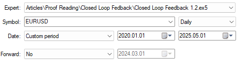
Figure 6: Backtesting the improved version of our feedback controller over the same time period

Our detailed statistics show clear and measurable growth over the initial version of the trading strategy. This improved version of the strategy, exposes us to less risk overall than the initial version of the trading strategy did. It is also interesting to note that the proportion of profitable short trades improved significantly, approaching almost 70%.

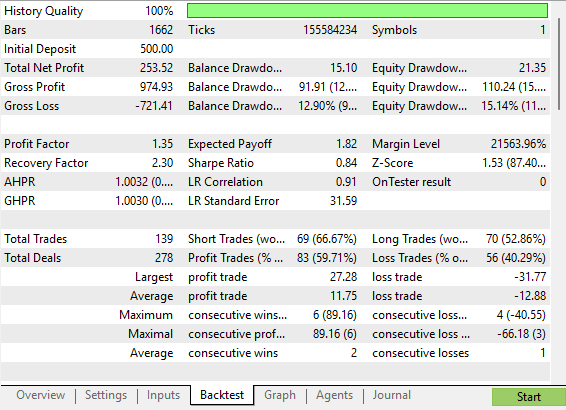
Figure 7: A detailed analysis of the improvements we have made to our trading system

Our new strategy produced an equity curve with fewer periods of drawdown when compared to the original strategy. This strategy shows steady growth that is less volatile, but still more rapid than the original risky version of our trading strategy.

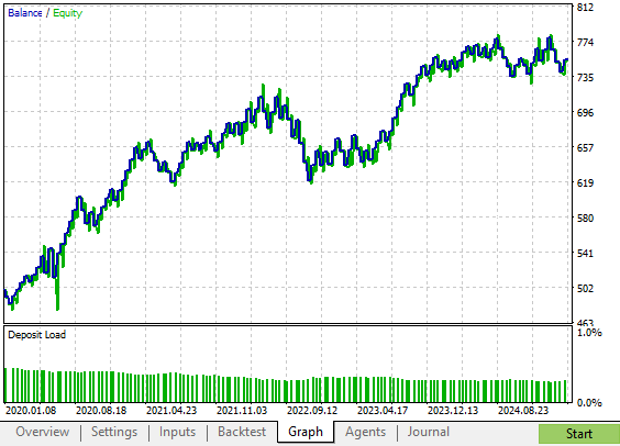
Figure 8: The equity curve produced by our improved version of the trading strategy shows us accelerated growth when compared to the original strategy

Conclusion

Imagine holding a golf ball at arm’s length against the sky and asking your AI model to compare its size to the Moon by eye. On some days, the model would decide the Moon is slightly bigger than the golf ball, and on others, it might claim the golf ball is slightly bigger than the Moon. As humans, we know such an activity is fundamentally flawed and, to a certain extent, humorous; however, the fun stops here.

In principle, our machine learning models may silently make the same error when trading financial markets. In the thought experiment, the error being made is that the model did not understand it was not working with the Moon directly—it is comparing an image of the Moon as projected in the sky.

And in the markets, our machine learning models are not predicting the “real” future price value; rather, they are creating images of the target onto the features. Therefore, we should not compare predictions made by our model directly to real prices as if they were the same. Instead, we must recognize that our machine learning models are trying to draw an image of the target, using a coordinate system learned from the inputs, and images are always separated from reality by some irreducible distance. That image can be distorted by many factors, so we should avoid relying on direct predictions.

Instead, after reading this article, the reader walks away empowered, knowing why we should use multiple forecast horizons to reduce the effect of this misalignment error, an error that usually goes unquestioned.