Neural Networks in Trading: An Ensemble of Agents with Attention Mechanisms (MASAAT)

Introduction

Portfolio management of financial instruments is a key component of investment decision-making, aimed at increasing returns while minimizing risks through the dynamic allocation of capital across assets. The high volatility of financial markets, where asset prices depend on a multitude of factors, complicates the construction of an optimal portfolio that simultaneously addresses two conflicting objectives: maximizing profits and minimizing risks. Traditional financial models, built on various investment principles, often prove effective in a single market but may fail under the complex and dynamic conditions of modern markets.

In recent years, growing attention has been given to machine learning methods for analyzing non-stationary price series. Among these, deep learning and reinforcement learning strategies have demonstrated notable success in computational finance. However, price data in financial markets are typically noisy time series, where extracting signals indicative of future trends is challenging.

One promising approach is presented in the paper "Developing an attention-based ensemble learning framework for financial portfolio optimisation". The authors introduce an innovative adaptive trading framework integrating attention mechanisms and time-series analysis (Multi-Agent and Self-Adaptive portfolio optimisation framework integrated with Attention mechanisms and Time series — MASAAT). Within this framework, multiple agents are deployed to observe and analyze directional changes in asset prices at varying levels of granularity. The goal is to enable thorough portfolio rebalancing to balance returns and risks in highly volatile markets.

By applying directional movement filters with different thresholds to capture significant price changes, the agents first extract trend features from raw time series. This allows them to track market regime shifts from multiple perspectives. Such an approach introduces a novel way of generating tokens in sequences, enabling the Cross-Sectional Attention (CSA) and Temporal Attention (TA) modules within the agents to effectively capture both asset correlations and temporal dependencies. Specifically, when reconstructing feature maps, sequence tokens in the CSA module are based on individual asset features, optimizing attention embeddings across assets, while tokens in the TA module are based on individual time points, capturing relevance between current and past observations.

Furthermore, information on asset and temporal dependencies is integrated within a spatio-temporal attention block. With clearly defined roles for CSA and TA, agents are equipped with richer insights into asset trends, allowing them to propose portfolios based on their unique perspectives. Ultimately, the portfolios generated by different agents are combined into a new ensemble portfolio that adapts dynamically to current market conditions. Even if a single agent misinterprets market trends and produces biased recommendations, the MASAAT framework, through its multi-agent integration, can adaptively refine the final portfolio to mitigate negative outcomes.

The MASAAT Algorithm

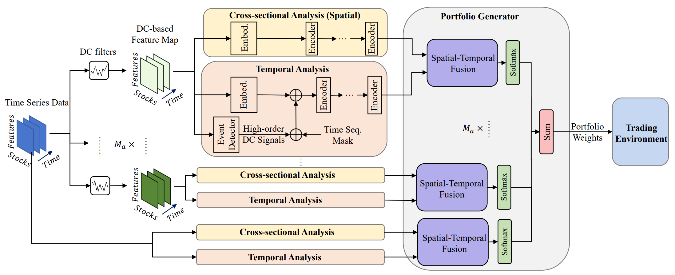
The MASAAT framework applies multiple directional movement filters with varying thresholds to capture significant price fluctuations across multi-scale receptive fields, enabling analysis of potential influences on future price movements. These receptive fields represent different levels of asset price volatility, giving agents an intuitive perception of market dynamics. By reconstructing asset-oriented directional movement features in the CSA module and time-point-oriented features in the TA module into sequence tokens, the multi-agent MASAAT framework simultaneously collects spatial and temporal information across different scales of price changes. This facilitates the identification of both the direction and magnitude of upcoming trends. Raw price series are directly transformed into asset- and time-oriented features, followed by cross-sectional and temporal analysis within the CSA and TA modules.

Notably, the CSA and TA modules are built on Self-Attention encoders, where attention scores are calculated across the entire sequence of tokens. This allows for a fair estimation of similarity across all assets, unlike convolutional neural networks (CNNs), which are highly sensitive to local positional structures in feature maps and rely on kernel sizes. By usig attention scores that explicitly quantify token similarities, the trading signals generated by MASAAT are inherently more interpretable. Through spatio-temporal attention blocks, mappings are constructed between asset sequences and historical time-point sequences. This process generates embeddings that represent each asset's attention scores across all time points within the observation window. These embeddings are then used to propose portfolio allocations. A portfolio generator consolidates agent-level proposals into a revised ensemble portfolio, enabling adaptive responses to evolving market conditions.

Let N be the number of assets, M the number of observable market features, and Ma the number of trading agents. For a given historical depth, each agent first observes price features 𝐏 ∈ RN×M×Tw over the observation window Tw. Then trend-based functions 𝐏DC={𝐏DC,1, 𝐏DC,2,…,𝐏DC,𝐌a} ∈ RMa, 𝐏DC,i ∈ RN×M×Tw are extracted using directional movement filters. As mentioned above, the method 𝐏DC,i are transformed into 𝐏DC,i,CSA ∈ RN×MTw for the module CSA and 𝐏DC,i,TA ∈ RTw×NM for the module ТА. The interdependences are then analyzed in the Transformer encoder. Similarly, the raw price series 𝐏 is transformed into 𝐏CSA ∈ RN×MTw and 𝐏TA ∈ RTw×NM.

After analyzing token dependencies, CSA and TA modules output asset-oriented embeddings 𝐎CSA ∈ RN×D and time-oriented embeddings 𝐎TA ∈ RTw×D, where D is the embedding vector dimension. These embeddings are merged to construct an updated portfolio, which is further integrated with outputs from other agents to obtain the final dependency vector W𝐭 and refine the portfolio.

After trading operations are executed, rewards rt are collected and stored in the experience replay buffer Ď, along with W𝐭, 𝐏 and 𝐏DC. Also, the Actor policy π is iteratively updated by sampling from Ď using a policy gradient method.

Since higher returns typically come with higher risks, diversification is both crucial and challenging. Agents must assign appropriate weights to heterogeneous assets to achieve hedging effects. Thus, continuously learning asset correlations allows agents to manage risks more effectively in turbulent market conditions.

The trend features are transformed into sequence tokens before correlation analysis through Self-Attention encoders. The optimized attention vector quantifies correlations between assets, where assets with similar attention vectors are inferred to share relevant characteristics.

Beyond asset correlation, MASAAT also investigates temporal relevance across observation windows, aiming to predict price trends at multiple levels. In this case, each time point is treated as a sequence token, and correlations between time points are learned through Transformer encoders. Two time points with similar attention vectors are considered to share comparable trend dynamics.

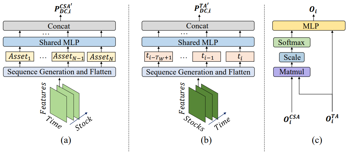
By aggregating information from CSA and TA modules, MASAAT agents combine asset-level and time-level attention scores, estimating each asset’s importance relative to each time point in the observation period. Each agent's proposed portfolio can be expressed as:

where 𝐕i and bi are learnable parameters of MLP.

The outputs of multiple agents, each observing price fluctuations at different granularities, are then integrated to form an ensemble portfolio responsive to the current financial environment. Compared to portfolios generated by individual agents, the multi-agent structure of MASAAT provides multiple candidate portfolios derived from diverse perspectives. This significantly enhances the system adaptability, particularly in highly volatile markets.

The original visualization of the MASAAT framework is provided below.

Implementation in MQL5

After discussing the theoretical aspects of the MASAAT framework, we now turn to the practical part of this article, where we present an implementation of our interpretation of the proposed approach using MQL5. As noted earlier, MASAAT is a comprehensive framework. To maintain a clear separation of functionality across different blocks, we will design it as a modular structure composed of independent objects, each responsible for part of the MASAAT functionality.

We begin with the trend detection mechanism. A piecewise linear representation (PLR) layer for time series is well-suited for identifying local trends. However, there is a limitation: the previously implemented object can only act as a single agent. Since MASAAT requires flexible functionality for building models with multiple agents, we need a more scalable solution.

One option would be to use a dynamic array containing pointers to several PLR objects of the analyzed time series, each operating with different threshold values. However, this approach leads to sequential execution, which is not optimal. Instead, we will develop a new object that enables parallel operation of multiple trend-detection agents. To achieve this, we first need to extend the OpenCL program with new kernels.

OpenCL Program Extension

When attempting to adapt the existing PLR kernels, we faced the need to replace a single threshold parameter with a vector of threshold values, one for each agent. This change requires not only modifying the kernel algorithm but also restructuring the dependent objects. To simplify development, we created new forward and backward pass kernels, partially reusing the logic of the existing implementation.

For the feed-forward pass, we developed the PLRMultiAgents kernel. It receives four data buffer pointers. Two buffers contain the raw time series and agent-specific threshold values. The other two buffers store the analysis results and trend-reversal flags.

__kernel void PLRMultiAgents(__global const float *inputs,
                             __global float *outputs,
                             __global int *isttp,
                             const int transpose,
                             __global const float *min_step
                            )
  {
   const size_t i = get_global_id(0);
   const size_t lenth = get_global_size(0);
   const size_t v = get_global_id(1);
   const size_t variables = get_global_size(1);
   const size_t a = get_global_id(2);
   const size_t agents = get_global_size(2);

This kernel is executed in a 3D task space. The first dimension corresponds to the size of the analyzed sequence. The second dimension corresponds to the number of univariate series in a multimodal sequence. The third dimension corresponds to the number of agents. Within the kernel, each thread identifies its position across all task dimensions. After that we determine the offset in the data buffers.

//--- constants
   const int shift_in = ((bool)transpose ? (i * variables + v) : (v * lenth + i));
   const int step_in = ((bool)transpose ? variables : 1);
   const int shift_ag = a * lenth * variables;

It is important to note that all agents analyze the same multimodal sequence. Thus, the agent identifier affects only the buffer offset for results and threshold values.

After initialization, the kernel begins searching for trend reversal points (extrema). Each flow determines the presence of a trend reversal point at the position of the current element. The extreme points of the analyzed time series automatically receive the status of a trend reversal point, since they are a priori the extreme points of the segment.

//--- look for ttp
   float value = IsNaNOrInf(inputs[shift_in], 0);
   bool bttp = false;
   if(i == 0 || i == lenth - 1)
      bttp = true;

For other points, the algorithm searches backward for the nearest element with a deviation exceeding the threshold. During this process, we record the minimum and maximum values in the checked interval.

   else
     {
      float prev = value;
      int prev_pos = i;
      float max_v = value;
      float max_pos = i;
      float min_v = value;
      float min_pos = i;
      while(fmax(fabs(prev - max_v), fabs(prev - min_v)) < min_step[a] && prev_pos > 0)
        {
         prev_pos--;
         prev = IsNaNOrInf(inputs[shift_in - (i - prev_pos) * step_in], 0);
         if(prev >= max_v && (prev - min_v) < min_step[a])
           {
            max_v = prev;
            max_pos = prev_pos;
           }
         if(prev <= min_v && (max_v - prev) < min_step[a])
           {
            min_v = prev;
            min_pos = prev_pos;
           }
        }

Search forward for the next element with the required deviation.

      float next = value;
      int next_pos = i;
      while(fmax(fabs(next - max_v), fabs(next - min_v)) < min_step[a] && next_pos < (lenth - 1))
        {
         next_pos++;
         next = IsNaNOrInf(inputs[shift_in + (next_pos - i) * step_in], 0);
         if(next > max_v && (next - min_v) < min_step[a])
           {
            max_v = next;
            max_pos = next_pos;
           }
         if(next < min_v && (max_v - next) < min_step[a])
           {
            min_v = next;
            min_pos = next_pos;
           }
        }

Determine whether the current element qualifies as an extremum.

      if(
         (value >= prev && value > next) ||
         (value > prev && value == next) ||
         (value <= prev && value < next) ||
         (value < prev && value == next)
      )
         if(max_pos == i || min_pos == i)
            bttp = true;
     }

But here we should remember that when searching for elements with the minimum required deviation, we could collect a corridor of values from several elements of the sequence that form a certain extremum plateau. Therefore, an element receives a flag only if it is an extremum in such a corridor. If there are several elements with the same value, we assign the extremum flag to the first of them.

We save the obtained flag and clear the output buffer. At the same time, we synchronize the workgroup flows.

   isttp[shift_in + shift_ag] = (int)bttp;
   outputs[shift_in + shift_ag] = 0;
   barrier(CLK_LOCAL_MEM_FENCE);

Subsequent steps are performed only by threads associated with confirmed trend reversals. The rest do not meet the set conditions and practically complete the operations.

First we determine the position of the current extremum. For this we count all preceding extrema based on the saved flags up to the analyzed position and save the position of the previous extremum from the source data buffer in a local buffer.

//--- calc position
   int pos = -1;
   int prev_in = 0;
   int prev_ttp = 0;
   if(bttp)
     {
      pos = 0;
      for(int p = 0; p < i; p++)
        {
         int current_in = ((bool)transpose ? (p * variables + v) : (v * lenth + p));
         if((bool)isttp[current_in + shift_ag])
           {
            pos++;
            prev_ttp = p;
            prev_in = current_in;
           }
        }
     }

Then we compute the parameters of the linear approximation for the segment.

//--- cacl tendency
   if(pos > 0 && pos < (lenth / 3))
     {
      float sum_x = 0;
      float sum_y = 0;
      float sum_xy = 0;
      float sum_xx = 0;
      int dist = i - prev_ttp;
      for(int p = 0; p < dist; p++)
        {
         float x = (float)(p);
         float y = IsNaNOrInf(inputs[prev_in + p * step_in], 0);
         sum_x += x;
         sum_y += y;
         sum_xy += x * y;
         sum_xx += x * x;
        }
      float slope = IsNaNOrInf((dist * sum_xy - sum_x * sum_y) / (dist > 1 ? (dist * sum_xx - sum_x * sum_x) : 1), 0);
      float intercept = IsNaNOrInf((sum_y - slope * sum_x) / dist, 0);

After that, we save the obtained values in the results buffer.

      int shift_out = ((bool)transpose ? ((pos - 1) * 3 * variables + v) : (v * lenth + (pos - 1) * 3)) + shift_ag;
      outputs[shift_out] = slope;
      outputs[shift_out + step_in] = intercept;
      outputs[shift_out + 2 * step_in] = ((float)dist) / lenth;
     }

Each obtained segment is characterized by 3 parameters:

• slope — the trend line angle,
• intercept — the line offset in the data space,
• dist — the normalized length of the segment.

Storing the sequence length as an integer value is not the best option in this case. Because for the efficient operation of the model, a normalized data presentation format is preferable. Therefore, we translate the integer segment size into a fraction of the length of the univariate sequence being analyzed. To do this, we divide the number of elements in the segment by the number of elements in the entire sequence of the univariate time series. In order not to fall into the "trap" of integer operations, we will first convert the number of elements in the segment from int to the float type.

Additionally, we will create a separate branch of operations for the last segment. At this stage, we do not know the number of segments that will be formed at any given point in time. Hypothetically, in extreme scenarios (e.g., small thresholds and high volatility), reversals may occur at nearly every element. Although unlikely, this case would significantly increase data volume. At the same time, we do not want to lose data.

Therefore, we proceed from a priori knowledge of the representation of time series in MQL5 and understanding the structure of the analyzed data: the latest data in time is at the beginning of our time series. Let's dwell on them in more detail. Data at the end of the analyzed sequence happened earlier in history and thus has less influence on subsequent events. Although we will not exclude such dependencies.

Therefore, to write the results, we use a data buffer size similar to the size of the input time series tensor. This allows us to write segments 3 times smaller than the sequence length (3 elements to write 1 segment). We expect that this volume is more than sufficient. However, if there are more segments, we merge the data of the last segments into 1 to avoid data loss.

   else
     {
      if(pos == (lenth / 3))
        {
         float sum_x = 0;
         float sum_y = 0;
         float sum_xy = 0;
         float sum_xx = 0;
         int dist = lenth - prev_ttp;
         for(int p = 0; p < dist; p++)
           {
            float x = (float)(p);
            float y = IsNaNOrInf(inputs[prev_in + p * step_in], 0);
            sum_x += x;
            sum_y += y;
            sum_xy += x * y;
            sum_xx += x * x;
           }
         float slope = IsNaNOrInf((dist * sum_xy - sum_x * sum_y) / (dist > 1 ? (dist * sum_xx - sum_x * sum_x) : 1),0);
         float intercept = IsNaNOrInf((sum_y - slope * sum_x) / dist, 0);
         int shift_out = ((bool)transpose ? ((pos - 1) * 3 * variables + v) : (v * lenth + (pos - 1) * 3)) + shift_ag;
         outputs[shift_out] = slope;
         outputs[shift_out + step_in] = intercept;
         outputs[shift_out + 2 * step_in] = IsNaNOrInf((float)dist / lenth, 0);
        }
     }
  }

In most cases, we expect to have fewer segments, and then the last elements of our result buffer will be filled with zero values.

As you can see, we do not use trainable parameters in the feed-forward pass algorithm. So, the backpropagation pass is reduced to error gradient distribution. This functionality is implemented in the PLRMultiAgentsGradient kernel.

All agents analyze the same time series. Therefore, gradients from all agents must be aggregated at the raw data level. Given the expected modest number of agents, we chose not to overcomplicate the kernel. Instead, we reuse the single-agent gradient distribution algorithm. However, we also add a loop to collect gradients from all agents and a parameter specifying their number. I encourage you to explore their implementations independently. The complete OpenCL program, including these kernels, is provided in the attachment.

Trend Detection Mechanism Object

Having completed the OpenCL-side implementation, we now move to our main library and implement the multi-agent trend detection algorithm within the object CNeuronPLRMultiAgentsOCL. As you may notice, this object essentially extends the previously developed piecewise linear representation (PLR) of a time series. This is why we selected it as the parent class. The structure of the new object is presented below.

class CNeuronPLRMultiAgentsOCL  :  public CNeuronPLROCL
  {
protected:
   int               iAgents;
   CBufferFloat      cMinDistance;
   //---
   virtual bool      feedForward(CNeuronBaseOCL *NeuronOCL);
   //---
   virtual bool      calcInputGradients(CNeuronBaseOCL *prevLayer);

public:
                     CNeuronPLRMultiAgentsOCL(void)  : iAgents(1) {};
                    ~CNeuronPLRMultiAgentsOCL(void) {};
   //---
   virtual bool      Init(uint numOutputs, uint myIndex, COpenCLMy *open_cl,
                          uint window_in, uint units_count, bool transpose,
                          vector<float> &min_distance,
                          ENUM_OPTIMIZATION optimization_type, uint batch);
   //---
   virtual int       Type(void)   const   {  return defNeuronPLRMultiAgentsOCL;   }
   //---
   virtual bool      Save(int const file_handle);
   virtual bool      Load(int const file_handle);
   virtual void      SetOpenCL(COpenCLMy *obj);
  };

In this new class, we declare a constant defining the number of active agents (iAgents) and a buffer for storing the threshold values of feature changes in the analyzed time series (cMinDistance).

Since all internal objects are declared statically, we can keep the constructor and destructor empty. The initialization of these declared and inherited objects is performed in the Init method.

bool CNeuronPLRMultiAgentsOCL::Init(uint numOutputs, uint myIndex, COpenCLMy *open_cl,
                                    uint window_in, uint units_count, bool transpose,
                                    vector<float> &min_distance,
                                    ENUM_OPTIMIZATION optimization_type, uint batch)
  {
   iAgents = (int)min_distance.Size();
   if(iAgents <= 0)
      return false;

Note that the method takes only a vector of threshold values as input. We do not explicitly pass the number of agents. The number is derived from the size of the threshold vector itself. This reduces the number of external parameters and guarantees consistency between the threshold parameter and the buffer length.

Within the method, after saving the agent count in an internal variable and validating it (at least one agent is required for proper operation), we call the initialization method of the base object, which sets up the core interfaces.

   if(!CNeuronBaseOCL::Init(numOutputs, myIndex, open_cl, window_in * units_count * iAgents, optimization_type, batch))
      return false;

Importantly, we call the base object's Init method, not the direct parent's one. This is because the size of the results buffer is scaled proportionally to the number of agents. However, this requires a deeper reinitialization of inherited components.

First, we save the values of the received parameters in inherited variables.

   iVariables = (int)window_in;
   iCount = (int)units_count;
   bTranspose = transpose;

And then we initialize the buffer of extremum flags.

   icIsTTP = OpenCL.AddBuffer(sizeof(int) * Neurons(), CL_MEM_READ_WRITE);
   if(icIsTTP < 0)
      return false;

Note that these flags are recalculated after every feed-forward pass. Their size matches that of the results buffer. Obviously, there is no need to store their values permanently. Thus, the buffer is created only in the OpenCL context memory. The object retains only a pointer to it.

Next we initialize the threshold buffer.

   if(!cMinDistance.AssignArray(min_distance) ||
      !cMinDistance.BufferCreate(OpenCL))
      return false;
//---
   return true;
  }

After that, we complete the method by returning the logical result of the initialization process to the calling program.

The feed-forward and backpropagation methods are also overridden. However, their sole function is to invoke the OpenCL kernels described earlier. Since their logic is straightforward, we leave them for independent study.

This concludes the implementation of the multi-agent trend detection object CNeuronPLRMultiAgentsOCL. The full source code of its methods is provided in the attachment.

Cross-Sectional Attention Module (CSA)

Once we obtain the multi-scale piecewise linear representations of the analyzed time series, each agent processes its assigned scale for in-depth analysis. Within the MASAAT framework, time series are analyzed in two projections: across assets and across time points.

Time series analysis within the MASAAT framework is performed by the module of cross-asset attention, which we implement as a CNeuronCrossSectionalAnalysis object. But before we get down to implementation, let's talk about the CSA module construction algorithm.

As explained in the theoretical section of MASAAT description, the CSA module uses a Self-Attention encoder to capture asset dependencies. Our library already contains several encoder implementations. However, there is a nuance: in MASAAT, multiple agents work in parallel, with each analyzing dependencies only within its assigned subset of the data. After review, we can identify a suitable solution.

Fore example, the CNeuronMVMHAttentionMLKV block for independent channel analysis, originally developed for the InjectTST framework. Not a bad solution. While this block is designed to analyze dependencies across multiple scales of a single asset, our task is to find dependencies between different assets within one scale. To adapt it, we first transpose the three-dimensional input tensor along its first two axes. We already have such a transposition layer in our library: CNeuronTransposeRCDOCL.

We've decided on the encoder. But before feeding data into the encoder, we also need to generate asset trajectory embeddings. The MASAAT authors suggest using an MLP with shared parameters across assets. Following our convention, we replace the MLP with a convolutional layer. Specifically, we add a single convolutional layer with GELU activation. The second MLP role (generating Query, Key, Value entities) is handled internally by the encoder itself.

This will be the structure of our CSA module. In it, we will successively use a data transposition layer, a convolutional embedding layer, and an independent channel analysis block (Self-Attention encoder). For efficiency, we place the convolutional layer before transposition. The result of the operations will not change. However, this positively affects the effectiveness of the solution.

We feed some representation of the time series with the price movements of the analyzed assets to the CSA module. Consequently, as the depth of the analyzed history increases, the volume of source data also increases. Since the PLR often contains many zero-filled elements, smaller embeddings can be used. This reduces the size of the tensor that needs to be transposed after the convolutional embedding layer operations, decreasing computational overhead and improving performance.

After identifying the key aspects of implementation, we can move on to constructing our new object CNeuronCrossSectionalAnalysis. Its structure is presented below.

class CNeuronCrossSectionalAnalysis :  public CNeuronMVMHAttentionMLKV
  {
protected:
   CNeuronConvOCL          cEmbeding;
   CNeuronTransposeRCDOCL  cTransposeRCD;
   //---
   virtual bool      feedForward(CNeuronBaseOCL *NeuronOCL) override;
   virtual bool      calcInputGradients(CNeuronBaseOCL *prevLayer) override;
   virtual bool      updateInputWeights(CNeuronBaseOCL *NeuronOCL) override;

public:
                     CNeuronCrossSectionalAnalysis(void) {};
                    ~CNeuronCrossSectionalAnalysis(void) {};
   //---
   virtual bool      Init(uint numOutputs, uint myIndex, COpenCLMy *open_cl,
                          uint window, uint window_key, uint heads, uint heads_kv,
                          uint units_count, uint layers, uint layers_to_one_kv,
                          uint variables, ENUM_OPTIMIZATION optimization_type, uint batch) override;
   //---
   virtual int       Type(void)   const override   {  return defNeuronCrossSectionalAnalysis;   }
   //---
   virtual bool      Save(int const file_handle) override;
   virtual bool      Load(int const file_handle) override;
   virtual bool      WeightsUpdate(CNeuronBaseOCL *source, float tau) override;
   virtual void      SetOpenCL(COpenCLMy *obj) override;
  };

Note that we use the Independent Channel Analysis block as the parent class. This solution allows us to reuse its methods directly rather than embedding it as an internal component. We declare other objects as static and thus we can leave the class constructor and destructor empty. Initialization is performed in the Init method, whose parameters mirror those of the parent class.

bool CNeuronCrossSectionalAnalysis::Init(uint numOutputs, uint myIndex, COpenCLMy *open_cl,
                                         uint window, uint window_key, uint heads, uint heads_kv,
                                         uint units_count, uint layers, uint layers_to_one_kv, uint variables,
                                         ENUM_OPTIMIZATION optimization_type, uint batch)
  {
   if(!CNeuronMVMHAttentionMLKV::Init(numOutputs, myIndex, open_cl, window_key, window_key, heads, heads_kv,
                                      variables, layers, layers_to_one_kv, units_count, optimization_type, batch))
      return false;

In the method body, as usual, we first call the relevant method of the parent class. There is one caveat. While implementing the CSA module functionality, we plan to make full use of all inherited methods. Within the feed-forward pass, the input of the parent class method will be fed with transposed embeddings of the raw data. Therefore, when calling the initialization method of the parent class, we resize the source data window to match the embedding dimension and swap the parameters of the analyzed sequence length with the number of independent variables.

After the initialization operations of the parent class objects have been successfully completed, we sequentially initialize the convolutional embedding and data transposition layer.

   if(!cEmbeding.Init(0, 0, OpenCL, window, window, window_key, units_count, variables, optimization, iBatch))
      return false;
   cEmbeding.SetActivationFunction(GELU);
   if(!cTransposeRCD.Init(0,1,OpenCL,variables,units_count,window_key,optimization,iBatch))
      return false;

After that, we forcibly disable the activation function and terminate the method, having previously returned the logical result of the operations to the calling program.

   SetActivationFunction(None);
//---
   return true;
  }

Next, we build the feed-forward pass algorithm of our CSA module in the feedForward method. Everything is quite straightforward here. In the method parameters, we receive a pointer to the input data object, which we immediately pass to the identically named method of the convolutional layer.

bool CNeuronCrossSectionalAnalysis::feedForward(CNeuronBaseOCL *NeuronOCL)
  {
   if(!cEmbeding.FeedForward(NeuronOCL))
      return false;
   if(!cTransposeRCD.FeedForward(cEmbeding.AsObject()))
     return false;
//---
   return CNeuronMVMHAttentionMLKV::feedForward(cTransposeRCD.AsObject());
  }

We transpose the outputs of the convolutional layer and pass them to the identically named method of the parent class. The method concludes by returning the logical result of the operation to the calling program.

The backpropagation algorithm is also simple. Therefore, I suggest you explore it independently. We complete our work on the CNeuronCrossSectionalAnalysis object. You can find the full code of all these methods in the attachment.

Our working day is now over. However, the work is not finished yet. Let's take a short break, and in the next article, we will bring the project to its logical conclusion.

Conclusion

In this article, we explored the Multi-Agent Self-Adaptive Attention-based Time Series framework (MASAAT) for portfolio optimization, which employs an ensemble of trading agents to analyze price data from multiple perspectives. This reduces the bias of generated trading actions. Each agent performs cross-sectional and temporal analyses using attention mechanisms to capture correlations between assets and time points, followed by a spatio-temporal fusion module to integrate the extracted information.

In the practical part, we began implementing our own interpretation of MASAAT in MQL5, including the multi-agent trend detection mechanism and the cross-sectional attention module. In the next article, we will continue this work and evaluate the performance of the implemented solution on real historical data.

References

• Developing An Attention-Based Ensemble Learning Framework for Financial Portfolio Optimisation
• Other articles from this series

Programs used in the article

#	Name	Type	Description
1	Research.mq5	Expert Advisor	Expert Advisor for collecting samples
2	ResearchRealORL.mq5	Expert Advisor	Expert Advisor for collecting samples using the Real-ORL method
3	Study.mq5	Expert Advisor	Model training Expert Advisor
4	Test.mq5	Expert Advisor	Model testing Expert Advisor
5	Trajectory.mqh	Class library	System state description structure
6	NeuroNet.mqh	Class library	A library of classes for creating a neural network
7	NeuroNet.cl	Code Base	OpenCL program code library