Neural Networks in Trading: A Multi-Agent Self-Adaptive Model (MASA)

Introduction

Computer technologies are becoming an integral part of financial analytics, offering innovative approaches to solving complex problems. In recent years, reinforcement learning (RL) has proven its effectiveness in dynamic portfolio management under the conditions of turbulent financial markets. However, existing methods often concentrate on maximizing returns while paying insufficient attention to risk management—particularly under uncertainty caused by pandemics, natural disasters, and regional conflicts.

To address this limitation, the study "Developing A Multi-Agent and Self-Adaptive Framework with Deep Reinforcement Learning for Dynamic Portfolio Risk Management" introduces MASA (Multi-Agent and Self-Adaptive). MASA integrates two interacting agents: the first optimizes returns using the TD3 algorithm, while the second minimizes risks through evolutionary algorithms or other optimization methods. In addition, MASA incorporates a market observer that leverages deep neural networks to analyze market trends and provide feedback.

The authors tested MASA on data from the CSI 300, Dow Jones Industrial Average (DJIA), and S&P 500 indices over the past 10 years. Their results demonstrate that MASA outperforms traditional RL-based approaches in portfolio management.

1. The MASA Algorithm

To overcome the limitations of conventional RL approaches, which tend to focus excessively on return optimization, the authors propose a multi-agent self-adaptive architecture (MASA). This structure employs two interactive and reactive agents (one based on RL, the other on an alternative optimization algorithm) to establish a fundamentally new multi-agent RL scheme. The objective is to dynamically balance the trade-off between portfolio returns and potential risks, particularly under volatile market conditions.

Within this architecture, the RL agent, built on the TD3 algorithm, optimizes overall portfolio returns. Simultaneously, the alternative optimization agent adapts the portfolio generated by the RL agent, minimizing risks after incorporating market trend assessments provided by the market observer.

This clear functional separation allows the model to continuously learn and adapt to the underlying dynamics of financial markets. As a result, MASA produces more balanced portfolios, both in terms of profitability and risk, compared to approaches based solely on RL.

Importantly, the MASA framework employs a loosely coupled, pipeline-like computational model across its three intelligent interacting agents. Thus, the general approach based on multi-agent RLensures resilience and robustness: the system continues operating effectively even if one of the agents fails.

Before the iterative training process begins, all relevant information is initialized, including the RL policy and the market state data maintained by the Market Observer agent.

During training, information about the current market state Ot (e.g., the most recent upward or downward trends in the underlying market over the past few trading days) is collected for analysis by the Market Observer. In parallel, the reward from the previously executed action At−1,Final is used as feedback for the RL algorithm to refine the RL agent behavior policy.

The Market Observer is then activated to compute the proposed risk boundary σs,t and the market vector Vm,t, which serve as additional features for updating both the RL agent and the Controller in response to current market conditions.

To ensure flexibility and adaptability, the MASA framework can incorporate a variety of approaches, including algorithmic models or deep neural networks. More importantly, both RL-based and alternative optimization-based agents are inherently safeguarded by continuous access to current market information, which provides the most valuable feedback from the trading environment. The insights generated by the Market Observer are used exclusively as auxiliary information, enabling faster adaptation and improved performance of both the RL agent and the Controller, particularly in highly volatile markets.

In worst-case scenarios, when the Market Observer generates misleading signals due to "noise", potentially affecting the other agents' decision-making, the adaptive nature of RL reward mechanism allows the system to re-align with the underlying trading environment during subsequent training iterations. Furthermore, the Market Observer's self-correcting capability over time helps mitigate the effects of misleading signals, ensuring stability across longer trading horizons.

Experimental results show that both RL-based agents and alternative optimizers demonstrate substantial performance improvements - even when the Market Observer is implemented with relatively simple algorithmic methods. This outcome highlights MASA's robustness when tested on complex datasets such as CSI 300, DJIA, and S&P 500 over a 10-year period.

Nevertheless, to fully understand the long-term impact of the Market Observer's input on the other two agents to which the proposed MASA framework should be applied, further analysis is required across more complex datasets and different application domains.

After the Market Observer is activated, the RL agent generates the current action At,RL in the form of portfolio weights. These weights may then be revised by the Controller, which applies an alternative optimization algorithm after considering its own risk management strategy as well as the market conditions identified by the Observer. Thanks to this loosely coupled, pipeline-based model, MASA functions as a robust Multi-Agent Aystem (MAS), maintaining operational integrity even if one agent fails.

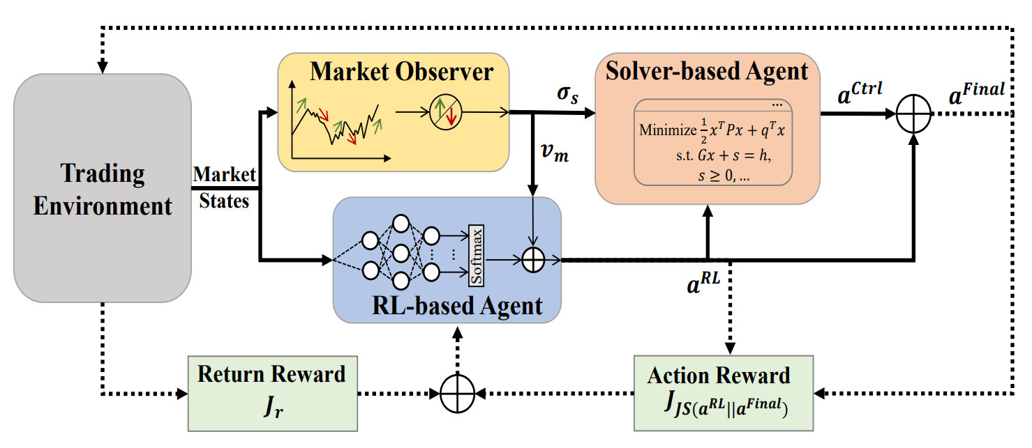
Guided by its reward-based mechanism, MASA adapts seamlessly to continuously evolving environments. The decision-making agents iteratively enhance portfolio performance with respect to both return and risk objectives, informed by valuable feedback from the Market Observer. Simultaneously, its reward mechanism incorporates an entropy-based divergence measure to encourage diversity in the set of generated actions as an intelligent and adaptive strategy essential for coping with the volatility of different financial markets.

The original visualization of the MASA framework is provided below.

2. Implementation in MQL5

After reviewing the theoretical aspects of the MASA method, we now move on to the practical part of the article, where we implement our interpretation of the proposed approaches using MQL5.

As mentioned earlier, the MASA framework consists of three agents. For better readability and clarity of code, we will create a separate object for each agent and later combine them into a unified structure.

2.1 Market Observer Agent

We begin by developing the Market Observer agent. The authors of MASA emphasize that a variety of algorithms can be applied for market analysis - ranging from simple analytical methods to advanced deep learning models. The primary task of the Market Observer is to identify key trends in order to forecast the most probable upcoming movements.

In our implementation, we use a hybrid approach. First, we apply a piecewise-linear representation algorithm to capture current market tendencies. Next, we analyze dependencies among the identified trends of individual univariate sequences using an attention module with relative positional encoding. Finally, at the output stage, we attempt to forecast the most probable market behavior over a defined planning horizon using an MLP.

This composite algorithm for the Market Observer is encapsulated in a new object CNeuronMarketObserver. Its structure is presented below.

class CNeuronMarketObserver   :  public CNeuronRMAT
  {
public:
                     CNeuronMarketObserver(void)   {};
                    ~CNeuronMarketObserver(void)   {};
   virtual bool      Init(uint numOutputs, uint myIndex, COpenCLMy *open_cl,
                          uint window, uint window_key, uint units_count,
                          uint heads, uint layers, uint forecast,
                          ENUM_OPTIMIZATION optimization_type, uint batch);
   //---
   virtual int       Type(void) override   const   {  return defNeuronMarketObserver; }
  };

The algorithm follows a linear structure. For such a structure, the CNeuronRMAT class designed to support small-scale linear models is a suitable parent class for our new object. This allows us to define the Market Observer's structure primarily within the Init initialization method. The main functionality is already handled by the parent class.

The parameters of the Init method specify the constants that define the architecture of the Market Observer agent. These include:

• window — the size of the vector describing a single sequence element (number of univariate time series);
• window_key — the dimensionality of internal attention components (Query, Key, Value);
• units_count — the historical depth of data used for analysis;
• heads — the number of attention heads;
• layers — the number of attention layers;
• forecast — the forecasting horizon for the upcoming movement.

bool CNeuronMarketObserver::Init(uint numOutputs, uint myIndex, COpenCLMy *open_cl,
                                 uint window, uint window_key, uint units_count,
                                 uint heads, uint layers, uint forecast,
                                 ENUM_OPTIMIZATION optimization_type, uint batch)
  {
//--- Init parent object
   if(!CNeuronBaseOCL::Init(numOutputs, myIndex, open_cl, window * forecast,
                                                   optimization_type, batch))
      return false;

Inside this method, we first invoke the initialization method of the base fully connected layer, which serves as the root parent class for all neural layers in our library. The parent class method provides the initialization of the basic interfaces of our object.

Two important points should be noted here: First, we call the base class initialization method, not the direct parent's. This is because the Market Observer's architecture significantly differs from that of its parent class.

Second, when invoking the parent initialization method, we specify the object size as the product of the planning horizon and the sequence element vector size. This matches the tensor we expect as the output of the Market Observer.

We then clear the dynamic array of pointers to internal objects:

//--- Clear layers' array
   cLayers.Clear();
   cLayers.SetOpenCL(OpenCL);

At this stage, the preparatory work is complete, and we can proceed to the actual construction of the Market Observer agent.

The model expects as input a multimodal time series represented as a sequence of vectors describing individual system states (in our case bars). To properly handle each univariate sequence, the incoming data must first be transposed.

//--- Tranpose input data
   int lay_count = 0;
   CNeuronTransposeOCL *transp = new CNeuronTransposeOCL();
   if(!transp ||
      !transp.Init(0, lay_count, OpenCL, units_count, window, optimization, iBatch) ||
      !cLayers.Add(transp))
     {
      delete transp;
      return false;
     }

Then we transform them into a piecewise-linear representation.

//--- Piecewise linear representation
   lay_count++;
   CNeuronPLROCL *plr = new CNeuronPLROCL();
   if(!plr ||
      !plr.Init(0, lay_count, OpenCL, units_count, window, false, optimization, iBatch) ||
      !cLayers.Add(plr))
     {
      delete plr;
      return false;
     }

To analyze dependencies between these univariate sequences, we use an attention module with relative positional encoding, parameterized with the required number of internal layers.

//--- Self-Attention for Variables
   lay_count++;
   CNeuronRMAT *att = new CNeuronRMAT();
   if(!att ||
      !att.Init(0, lay_count, OpenCL, units_count, window_key, window, heads, layers,
                                                                optimization, iBatch) ||
      !cLayers.Add(att))
     {
      delete att;
      return false;
     }

Based on the outputs of the attention block, we try to predict the upcoming values for each univariate sequence. Here, we use a residual convolutional block (CResidualConv) as an MLP substitute for independently predicting values of each univariate time series.

//--- Forecast mapping
   lay_count++;
   CResidualConv *conv = new CResidualConv();
   if(!conv ||
      !conv.Init(0, lay_count, OpenCL, units_count, forecast, window, optimization, iBatch) ||
      !cLayers.Add(conv))
     {
      delete conv;
      return false;
     }

Finally, the predicted results are transformed back into the dimensionality of the original input data.

//--- Back transpose forecast
   lay_count++;
   transp = new CNeuronTransposeOCL();
   if(!transp ||
      !transp.Init(0, lay_count, OpenCL, window, forecast, optimization, iBatch) ||
      !cLayers.Add(transp))
     {
      delete transp;
      return false;
     }

To minimize data-copying operations, we apply a pointer substitution technique with external interface buffers for efficient memory management.

   if(!SetOutput(transp.getOutput(), true) ||
      !SetGradient(transp.getGradient(), true))
      return false;
//---
   return true;
  }

The method then concludes by returning the boolean result of the operation to the caller.

The core functionality of this class is inherited from its parent object. Therefore, the Market Observer agent is now complete. The full source code of this class is provided in the attachment.

2.2 RL Agent

The next step is building the RL agent. In the MASA framework, this agent operates in parallel with the Market Observer, conducting independent market analysis and making decisions based on its learned policy.

The MASA authors suggest implementing the RL agent with a TD3-based model. However, we take a different architecture of the RL agent. For independent environment analysis, we use the PSformer framework. Decision-making based on the performed analysis is handled by a lightweight perceptron enhanced with SAM optimization.

Our RL agent is implemented in a new object CNeuronRLAgent. Its structure is shown below.

class CNeuronRLAgent :  public   CNeuronRMAT
  {
public:
                     CNeuronRLAgent(void) {};
                    ~CNeuronRLAgent(void) {};
   //---
   virtual bool      Init(uint numOutputs, uint myIndex, COpenCLMy *open_cl,
                          uint window, uint units_count, uint segments, float rho,
                          uint layers, uint n_actions,
                          ENUM_OPTIMIZATION optimization_type, uint batch);
   //---
   virtual int       Type(void)   const   override {  return defNeuronRLAgent;   }
  };

Similar to the Market Observer, we use here inheritance from CNeuronRMAT, a linear model base class. Thus, we just need to specify the new module's architecture within the Init method.

bool CNeuronRLAgent::Init(uint numOutputs, uint myIndex, COpenCLMy *open_cl,
                          uint window, uint units_count, uint segments,
                          float rho, uint layers, uint n_actions,
                          ENUM_OPTIMIZATION optimization_type, uint batch)
  {
//--- Init parent object
   if(!CNeuronBaseOCL::Init(numOutputs, myIndex, open_cl, n_actions, optimization_type, batch))
      return false;

The method parameters are very similar to those of the Market Observer. However, there are some differences. For example, the forecast horizon parameter is replaced by the agent's action space (n_actions). Also, additional parameters include segments (number of segments) and rho (blurring coefficient).

Inside the Init method, we call the base fully connected layer initializer, specifying the action space of our RL agent as the output tensor size.

We then clear the dynamic array of internal object pointers.

//--- Clear layers' array
   cLayers.Clear();
   cLayers.SetOpenCL(OpenCL);

The model's input data is first passed into the PSformer, whose required number of layers is created within a loop.

//--- State observation
   int lay_count = 0;
   for(uint i = 0; i < layers; i++)
    {
     CNeuronPSformer *psf = new CNeuronPSformer();
     if(!psf ||
        !psf.Init(0, lay_count, OpenCL, window, units_count, segments, rho, optimization,iBatch)||
        !cLayers.Add(psf))
       {
        delete psf;
        return false;
       }
     lay_count++;
    }

The RL agent then makes decisions on the optimal action by feeding the outputs of the performed analysis into a decision block composed of convolutional and fully connected layers. The convolutional layer reduces dimensionality.

   CNeuronConvSAMOCL *conv = new CNeuronConvSAMOCL();
   if(!conv ||
      !conv.Init(n_actions, lay_count, OpenCL, window, window, 1, units_count,
                                                      1, optimization, iBatch) ||
      !cLayers.Add(conv))
     {
      delete conv;
      return false;
     }
   conv.SetActivationFunction(GELU);
   lay_count++;

The fully connected layer generates the action tensor.

   CNeuronBaseSAMOCL *flat = new CNeuronBaseSAMOCL();
   if(!flat ||
      !flat.Init(0, lay_count, OpenCL, n_actions, optimization, iBatch) ||
      !cLayers.Add(flat))
     {
      delete flat;
      return false;
     }
   SetActivationFunction(SIGMOID);

Note that in this case we do not use the Actor's stochastic policy. However, we may still need to use in the future, which we will discuss later.

By default, the action vector uses a sigmoid activation function, constraining values to the range between 0 and 1. This can be overridden by an external program if needed.

As before, we substitute pointers to data buffers of external interfaces, then return the Boolean result of initialization.

   if(!SetOutput(flat.getOutput(), true) ||
      !SetGradient(flat.getGradient(), true))
      return false;
//---
   return true;
  }

With this, the RL agent object is complete. The full code of this class and all its methods can be found in the attachment.

2.3 Controller

We have constructed objects of two agents out of three. We now turn to the third component: the Controller Agent. Its role is to assess risk and adjust the RL agent's actions based on the environment state analysis performed by the Market Observer.

The key distinction here is that the Controller processes two input data sources. It must evaluate not only each input individually but also their interdependencies. In my opinion, the Transformer decoder structure perfectly suits this task. Instead of standard Self-Attention and Cross-Attention modules, however, we use relative positional encoding variants.

The Controller is implemented as a new object CNeuronControlAgent again inheriting from CNeuronRMAT. Since it works with dual input streams, several methods require redefinition. The structure of the new class is shown below.

class CNeuronControlAgent  :  public CNeuronRMAT
  {
protected:
   virtual bool      feedForward(CNeuronBaseOCL *NeuronOCL) override { return false; }
   virtual bool      feedForward(CNeuronBaseOCL *NeuronOCL, 
                                 CBufferFloat *SecondInput) override;
   virtual bool      calcInputGradients(CNeuronBaseOCL *NeuronOCL) override { return false; }
   virtual bool      calcInputGradients(CNeuronBaseOCL *NeuronOCL, 
                                        CBufferFloat *SecondInput, 
                                        CBufferFloat *SecondGradient, 
                                        ENUM_ACTIVATION SecondActivation = None) override;
   virtual bool      updateInputWeights(CNeuronBaseOCL *NeuronOCL) override { return false; }
   virtual bool      updateInputWeights(CNeuronBaseOCL *NeuronOCL, 
                                        CBufferFloat *SecondInput) override;

public:
                     CNeuronControlAgent(void) {};
                    ~CNeuronControlAgent(void) {};
   //---
   virtual bool      Init(uint numOutputs, uint myIndex, COpenCLMy *open_cl,
                          uint window, uint window_key, uint units_count, uint heads,
                          uint window_kv, uint units_kv, uint layers,
                          ENUM_OPTIMIZATION optimization_type, uint batch);
   //---
   virtual int       Type(void) override   const   {  return defNeuronControlAgent; }
  };

Again, initialization of internal objects is performed in the Init method, which specifies the Transformer decoder architecture.

bool CNeuronControlAgent::Init(uint numOutputs, uint myIndex, COpenCLMy *open_cl,
                               uint window, uint window_key, uint units_count,
                               uint heads, uint window_kv, uint units_kv, uint layers,
                               ENUM_OPTIMIZATION optimization_type, uint batch)
  {
//--- Init parent object
   if(!CNeuronBaseOCL::Init(numOutputs, myIndex, open_cl, window * units_count, 
                                                     optimization_type, batch))
      return false;
//--- Clear layers' array
   cLayers.Clear();
   cLayers.SetOpenCL(OpenCL);

As in previous cases, we call the relevant method of the base fully connected layer, specifying the dimensionality of the outputs at the level of the main input tensor. After that, we clear the dynamic array of pointers.

Next, we proceed to construct the architecture of our Controller Agent. Recall that the Market Observer outputs a multimodal time series, a sequence of vectors representing predicted states of the environment (bars).

Two approaches are possible: aligning RL agent actions with individual bars, or with univariate sequences. We understand that the Market Observer provided us with only forecast data, the probability of which being realized is far from 100%. Also, there is a possibility of deviations in absolutely all values.

Let's think logically. How much information can the vector describing one forecast candlestick give us, provided that each element can cave varying deviations? The question is controversial and difficult to answer without understanding the accuracy of individual forecasts.

On the other hand, if you look at a separate univariate series, then, in addition to individual values, you can also identify the trend of the upcoming movement. Since the trend is formed by a set of values, we could logically expect the confirmation of a trend, even if some elements deviate.

Moreover, all univariate sequences in our multimodal time series have certain interdependencies. So, when the predicted trend of one univariate time series is confirmed by the values of another, the probability of such a forecast increases.

Taking this into account, we decided to analyze the dependence of the agent's actions on the predicted values of univariate sequences. Accordingly, we first feed the secondary data source into a prepared neural layer.

   int lay_count = 0;
   CNeuronBaseOCL *flat = new CNeuronBaseOCL();
   if(!flat ||
      !flat.Init(0, lay_count, OpenCL, window_kv * units_kv, optimization, iBatch) ||
      !cLayers.Add(flat))
     {
      delete flat;
      return false;
     }

And then we reformat it into univariate sequence representations.

   lay_count++;
   CNeuronTransposeOCL *transp = new CNeuronTransposeOCL();
   if(!transp ||
      !transp.Init(0, lay_count, OpenCL, units_kv, window_kv, optimization, iBatch) ||
      !cLayers.Add(transp))
     {
      delete transp;
      return false;
     }
   lay_count++;

Next, we need to construct the architecture of our decoder. The required number of layers is created in a loop. The number of iterations is determined by the external parameters of the initialization method.

//--- Attention Action To Observation
   for(uint i = 0; i < layers; i++)
     {
      if(units_count > 1)
        {
         CNeuronRelativeSelfAttention *self = new CNeuronRelativeSelfAttention();
         if(!self ||
            !self.Init(0, lay_count, OpenCL, window, window_key, units_count, heads,
                                                               optimization, iBatch) ||
            !cLayers.Add(self))
           {
            delete self;
            return false;
           }
         lay_count++;
        }

It is important to note that, in the vanilla Transformer decoder, input data is first processed by a Self-Attention module, which analyzes dependencies between individual elements of the source sequence. In our implementation, we replace this module with its counterpart that uses relative positional encoding. However, we only create this module if the source sequence contains more than one element. Because, clearly, with only a single element, there are no dependencies to analyze. In this case, the Self-Attention module would be redundant.

Next, we create a Cross-Attention module, which analyzes dependencies between elements of the two data sources.

      CNeuronRelativeCrossAttention *cross = new CNeuronRelativeCrossAttention();
      if(!cross ||
         !cross.Init(0, lay_count, OpenCL, window, window_key, units_count, heads, 
                                        units_kv, window_kv, optimization, iBatch) ||
         !cLayers.Add(cross))
        {
         delete cross;
         return false;
        }
      lay_count++;

Each decoder layer is then completed with a FeedForward block, for which we use a residual convolutional block.

      CResidualConv *ffn = new CResidualConv();
      if(!ffn ||
         !ffn.Init(0, lay_count, OpenCL, window, window, units_count, optimization, iBatch) ||
         !cLayers.Add(ffn))
        {
         delete ffn;
         return false;
        }
      lay_count++;
     }

After this, we proceed to the next loop iteration and construct the following decoder layer.

As in the standard Transformer decoder architecture, the output of the residual convolutional block undergoes normalization. However, we may also need to constrain the Actor's action space to a defined range, which is typically handled by an activation function. Therefore, after constructing the required number of decoder layers, we add an additional convolutional layer with the specified activation function.

   CNeuronConvSAMOCL *conv = new CNeuronConvSAMOCL();
   if(!conv ||
      !conv.Init(0, lay_count, OpenCL, window, window, window, units_count, 1,
                                                       optimization, iBatch) ||
      !cLayers.Add(conv))
     {
      delete conv;
      return false;
     }
   SetActivationFunction(SIGMOID);

By default, as with the RL agent, we use the sigmoid function. However, we keep the option to override it from an external program.

Finally, at the end of the initialization method, we substitute pointers to the interface buffers and return a Boolean value to the calling program, indicating the success of the operation.

//---
   if(!SetOutput(conv.getOutput(), true) ||
      !SetGradient(conv.getGradient(), true))
      return false;
//---
   return true;
  }

After completing the initialization of the new object, we move on to constructing feed-forward algorithm in the feedForward method.

bool CNeuronControlAgent::feedForward(CNeuronBaseOCL *NeuronOCL, CBufferFloat *SecondInput)
  {
   if(!SecondInput)
      return false;

In the method parameters, we receive pointers to two input data objects. The primary data stream is passed as a neural layer, and the secondary data stream is provided as a data buffer. For ease of use, we substitute the buffer of results of a specially created internal layer with the object received in the method parameters.

   CNeuronBaseOCL *second = cLayers[0];
   if(!second)
      return false;
   if(!second.SetOutput(SecondInput, true))
      return false;

We then transpose the tensor of the secondary data source to represent the multimodal time series as a sequence of univariate series.

   second = cLayers[1];
   if(!second || !second.FeedForward(cLayers[0]))
      return false;

Next, we iterate through the remaining internal neural layers in sequence, calling their feed-forward methods and passing them both data sources.

   CNeuronBaseOCL *first = NeuronOCL;
   CNeuronBaseOCL *main = NULL;
   for(int i = 2; i < cLayers.Total(); i++)
     {
      main = cLayers[i];
      if(!main ||
         !main.FeedForward(first, second.getOutput()))
         return false;
      first = main;
     }
//---
   return true;
  }

After successfully completing all loop iterations, we simply return a Boolean result to the caller, signaling successful execution.

As can be seen, the feed-forward algorithm is relatively straightforward. This is thanks to the use of prebuilt blocks to construct a more complex architecture.

The situation becomes more challenging when implementing the error gradient distribution algorithm, due to the use of a secondary data source. Along the primary data path, information is passed sequentially from one internal layer to the next. However, the secondary data source is shared across all decoder layers. Specifically across all Cross-Attention modules. Consequently, the error gradient for the secondary data must be collected from all Cross-Attention modules. I suggest looking at the solution to this issue in code.

This logic is implemented in the calcInputGradients method. The method parameters include pointers to the two input data streams and their corresponding error gradients. Our task is to distribute the error gradient between the two data sources according to their contribution to the final output.

bool CNeuronControlAgent::calcInputGradients(CNeuronBaseOCL *NeuronOCL, CBufferFloat *SecondInput,
                              CBufferFloat *SecondGradient, ENUM_ACTIVATION SecondActivation = -1)
  {
   if(!NeuronOCL || !SecondGradient)
      return false;

Inside the method, we first validate the received pointers, since we cannot pass data to non-existent objects.

As with the forward pass, the secondary data source is represented as buffers. And we substitute the pointers in the corresponding internal layer.

   CNeuronBaseOCL *main = cLayers[0];
   if(!main)
      return false;
   if(!main.SetGradient(SecondGradient, true))
      return false;
   main.SetActivationFunction(SecondActivation);
//---
   CNeuronBaseOCL *second = cLayers[1];
   if(!second)
      return false;
   second.SetActivationFunction(SecondActivation);

At this stage, we also synchronize the activation functions of the internal layer and the subsequent transposition layer with the activation function of the input data. This ensures correct gradient propagation.

The transposition layer now acts as the secondary data source. For convenience, we store pointers to its interface objects in local variables.

   CBufferFloat *second_out = second.getOutput();
   CBufferFloat *second_gr = second.getGradient();
   CBufferFloat *temp = second.getPrevOutput();
   if(!second_gr.Fill(0))
      return false;

And we clear its gradient buffer of any previously accumulated values.

We then iterate backward through the internal neural layers. Note that within this loop we only work with decoder objects.

Since the first two internal objects are reserved for handling the secondary data source.

   for(int i = cLayers.Total() - 2; i >= 2; i--)
     {
      main = cLayers[i];
      if(!main)
         return false;

For each decoder layer, we retrieve its pointer from the array and validate it.

Because not all decoder modules operate with two data sources, the algorithm branches depending on the object type. For Cross-Attention modules, we first pass the error gradient of the secondary data source from the current layer into a temporary storage buffer, then accumulate these values with previously stored results.

      if(cLayers[i + 1].Type() == defNeuronRelativeCrossAttention)
        {
         if(!main.calcHiddenGradients(cLayers[i + 1], second_out, temp, SecondActivation) ||
            !SumAndNormilize(temp, second_gr, second_gr, 1, false, 0, 0, 0, 1))
            return false;
        }

For other modules, we simply propagate the error gradient along the primary path. And then we move on to the next iteration of the loop.

      else
        {
         if(!main.calcHiddenGradients(cLayers[i + 1]))
            return false;
        }
     }

After completing all iterations, we propagate the accumulated gradients back to the input data sources. First, we pass the gradient along the primary path to the first data source.

   if(!NeuronOCL.calcHiddenGradients(main.AsObject(), second_out, temp, SecondActivation))
      return false;

However, recall that the first decoder layer may be either a Self-Attention or Cross-Attention module. In the latter case, both data sources are used. So, we must check the object type and, if necessary, add the accumulated gradient of the second data source.

   if(main.Type() == defNeuronRelativeCrossAttention)
     {
      if(!SumAndNormilize(temp, second_gr, second_gr, 1, false, 0, 0, 0, 1))
         return false;
     }

Finally, we pass the complete accumulated gradient along the secondary path to the corresponding input source.

   main = cLayers[0];
   if(!main.calcHiddenGradients(second.AsObject()))
      return false;
//---
   return true;
  }

The method ends by returning a logical result to the calling program.

The parameter update algorithm, implemented in the updateInputWeights method, is relatively simple. We loop through the internal objects containing trainable parameters, calling their corresponding update methods. We will not go into detail here. But it is important to note that the constructed object architecture uses modules with SAM-optimized parameters. Therefore, the iteration through internal objects must be performed in reverse order.

With this, we conclude our discussion of the algorithms used to implement the Controller agent's methods. The complete code for the new class and all its methods is provided in the attachments.

We have made substantial progress today, though our work is not yet finished. We will take a short break, and in the next article, we will bring the project to its logical conclusion.

Conclusion

We have examined an innovative approach to portfolio management under volatile financial market conditions – the Multi-Agent Self-Adaptive (MASA) framework. The proposed framework successfully combines the advantages of RL algorithms for return optimization, adaptive optimization methods for risk minimization, and a Market Observer module for trend analysis.

In the practical section, we implemented each of the proposed agents in MQL5 as standalone modules. In the next article, we will integrate them into a complete system and evaluate the performance of the implemented solutions using real historical data.

References

• Developing A Multi-Agent and Self-Adaptive Framework with Deep Reinforcement Learning for Dynamic Portfolio Risk Management
• Other articles from this series

Programs used in the article

#	Name	Type	Description
1	Research.mq5	Expert Advisor	Expert Advisor for collecting examples
2	ResearchRealORL.mq5	Expert Advisor	Expert Advisor for collecting examples using the Real-ORL method
3	Study.mq5	Expert Advisor	Model training Expert Advisor
4	Test.mq5	Expert Advisor	Model testing Expert Advisor
5	Trajectory.mqh	Class library	System state description structure
6	NeuroNet.mqh	Class library	A library of classes for creating a neural network
7	NeuroNet.cl	Library	OpenCL program code library