Self Optimizing Expert Advisors in MQL5 (Part 13): A Gentle Introduction To Control Theory Using Matrix Factorization

Financial markets can often prove difficult to plan for or anticipate in advance. Investor sentiment is often fragile and can shift quickly depending on the global climate and the pressing issues dominating current affairs. Therefore, trading strategies that appear profitable in a historical context can often fall apart when deployed in real-time markets.

There are many reasons we can use to explain this behavior in trading applications. However, one key understanding is that once our applications have been developed and deployed, their behavior remains fixed and cannot usually be modified without human intervention. This means our strategies are vulnerable to repeating the same mistakes over and over again without ever profiting from failure or learning from past mistakes.

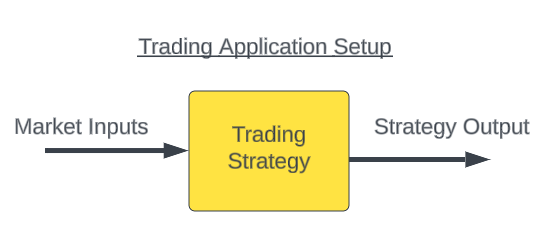
Figure 1: The normal trading setup used to deploy trading applications in finacnial markets

There have been many proposed solutions to this recurring problem. However, one solution that holds great potential comes from the field of control theory. Control theory is primarily concerned with correcting the behavior of a system operating in a dynamic or chaotic environment, with the goal of realigning the system toward a defined objective.

By periodically feeding back a copy of our strategy’s performance to a feedback controller—one that records and observes how the strategy interacts with the markets—we may be able to approximate the relationship between our strategy’s behavior and market outcomes. This controller aims to identify dominant patterns correlated with both losing trades and winning trades. If such a structure exists, and we can learn from it, then in theory the feedback controller should be able to modify and guide the dynamics of our trading system toward profitability, even during chaotic and ever-changing market conditions. 

This will effectively change out strategy's deployment structure from the schematic diagram depicted in Figure 1. In figure 2, we introduce the reader to simple notation used in control thoery literature and denoted the market's input signals as (M) and our strategy's outputs are denoted as (S).

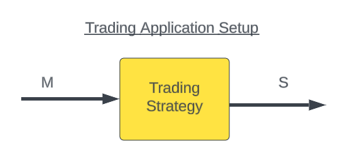
Figure 2: We can redifine our trading application using shorthand notation to represent the market inputs (M), and the strategy output (S)

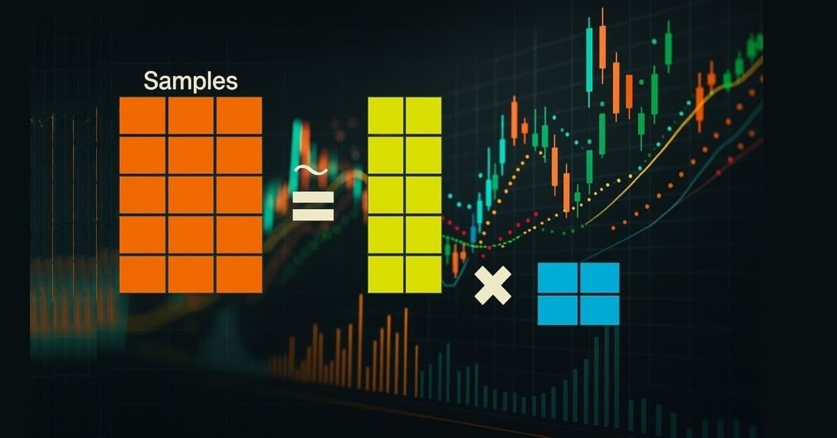
In most of our previous discussions on matrix factorization, we primarily focused on building regression and classification models to anticipate future price levels or changes in technical indicators. However, in this discussion we lean into control theory—specifically, a branch known as closed-loop feedback controllers. This area is often overlooked in discussions of numerically driven trading applications, even though its foundational theories can be extended to meet our needs as traders.

Our objective is to prove that feedback controllers provide a valuable level of fine control over trading systems. When carefully set up, these controllers can correct the system and keep it on track for profitable trades.

We began with the baseline version of our trading strategy, which employed two moving averages: one on the high price and the other on the low price. Both moving averages shared the same period, effectively creating a moving average channel. When price broke above this channel, we entered long positions; when price broke below the channel, we entered short positions. This baseline version set the profitability threshold we aimed to surpass with our feedback controller. Our trading strategy is illustrated below in Figure 3.

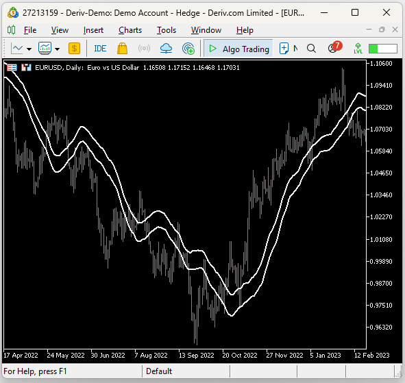
Figure 3: Visualizing our trading strategy in action on the EURUSD daily chart

Our feedback controller first observed our strategy’s performance over a 90-day period before being allowed to intervene. That is, during the first 90 days, the controller gave no input to the system and only gathered observations. Readers should note that this 90-day period is a tuning parameter, though the appropriate value is not always known in advance. We chose 90 days arbitrarily, assuming it would align with the business cycles of the financial institutions dominating forex markets. However, readers are free to experiment with this parameter as they see fit.

Over the course of those 90 days, the controller recorded several key variables: offered market prices, account balance, account equity, indicator values, and the types of positions we opened. These observations were stored in a matrix, referred to as a snapshot. We then fit a linear model that learned how snapshots evolved over time. In other words, the first 89 snapshots were mapped to the last 89 snapshots, teaching the system how the state of the strategy transitioned over time.

After 90 days, the linear system gathered all system states and predicted whether the next trade would be profitable or unprofitable. If the next trade was predicted to be unprofitable, the system simply paused trading until better market conditions were expected.

Therefore, the task of our feedback controller is to observe the outputs of our system (S) and learn a new control function(F) that modifies our system's behiavour (FS) to guide our system back to profitability so that our strategy isn't just being controlled directly by the market (M). After our 90-day observation period has elapsed, our strategy is no longer controlled by just the market (M), rather our strategy will now be controlled by a combination of the market inputs and the suggestions from our feedback controller (FS + M)

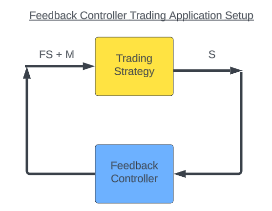
Figure 4: Visualizing how exactly our feedback controller will modify the behavior of our trading application after being deployed

We backtested both systems over five years of daily EUR/USD data. The feedback controller improved system profitability by 82%. Initially, our baseline strategy produced a profit of $134. After adding the feedback controller, profits rose to $245. Furthermore, the improved system realized these profits while taking fewer trades: the number of positions fell from 180 to 152—a 15% reduction in trading activity. This meant our new system generated higher profits while taking on less risk, a highly desirable feature for any trading application.

Additionally, overall risk was reduced. The baseline system accumulated a gross loss of –$1,092, while the feedback-controlled system reduced gross loss to –$838, all while maintaining nearly constant gross profit. This is another highly desirable outcome.

The Sharpe ratio of the baseline system was 0.34. After introducing the feedback controller, it increased to 0.68—a 100% improvement, which is remarkable for a market as challenging as EUR/USD. The ratio of profitable trades also rose by 6%, from 53.89% to 57.24%. Consequently, the proportion of losing trades fell by the same margin, showing that the feedback controller successfully learned dominant patterns that distinguished losing trades from winning ones. Lastly, the expected payoff increased from 0.75 to 1.61, representing a 114% improvement.

It is clear that feedback controllers can play a critical role in numerically driven trading applications. When configured correctly, they can reliably learn to intervene and prevent a strategy from repeating the same mistakes. Building a controller directly from snapshot observations is a technique known as system identification. 

These family of algorithms were initially developed by engineers interested in fluid dynamics. These engineers often found themselves trying to design controllers for the components that comprise the wings of aircrafts, however there are no explicit formulas for anticipating or correcting the effects of turbulence. Naturally, they needed to uncover methods for learning optimal control inputs from observations of the system’s behavior and the inputs that brought about that behavior. 

In our discussion, we built a linear model of the system, therefore this approach is more specifically called linear system identification. The results we present here motivate us to invest more time in assigning additional tasks to the feedback controller and to explore nonlinear system identifiers in the future. Let us get started.

Getting Started In MQL5

As with most of our trading applications, we begin by first defining important system definitions. For our baseline strategy, we only need one system definition, which sets the shared moving average period. 

//+------------------------------------------------------------------+
//|                                         Closed Loop Feedback.mq5 |
//|                                               Gamuchirai Ndawana |
//|                    https://www.mql5.com/en/users/gamuchiraindawa |
//+------------------------------------------------------------------+
#property copyright "Gamuchirai Ndawana"
#property link      "https://www.mql5.com/en/users/gamuchiraindawa"
#property version   "1.00"

//+------------------------------------------------------------------+
//| System definitions                                               |
//+------------------------------------------------------------------+
#define MA_PERIOD 10

The next important aspect of our system design is the set of global variables. For this particular baseline, we only need a handful of global variables tied to the technical indicators we rely on. Specifically, we will have handlers for the two moving average indicators and another handler for the ATR, which we use to set stop losses. Each of these indicators also requires its own dedicated buffer.

//+------------------------------------------------------------------+
//| Global variables                                                 |
//+------------------------------------------------------------------+
int    ma_h_handler,ma_l_handler,atr_handler;
double ma_h[],ma_l[],atr[];

Almost all trading applications we build in these discussions have dependencies, because we do not always write every piece of code from scratch. In this application, we call upon the trade library, as well as two custom libraries: one for keeping track of the formation of new candles, and another for retrieving key pricing information such as the bid and ask prices. 

//+------------------------------------------------------------------+
//| Dependencies                                                     |
//+------------------------------------------------------------------+
#include <Trade\Trade.mqh>
#include <VolatilityDoctor\Time\Time.mqh>
#include <VolatilityDoctor\Trade\TradeInfo.mqh>

CTrade      Trade;
Time        *DailyTimeHandler;
TradeInfo   *TradeInfoHandler;

When the system is initialized, we begin by creating new instances of our custom-defined classes. We also create new instances of our indicators. 

//+------------------------------------------------------------------+
//| Expert initialization function                                   |
//+------------------------------------------------------------------+
int OnInit()
  {
//---
   DailyTimeHandler = new Time(Symbol(),PERIOD_D1);
   TradeInfoHandler = new TradeInfo(Symbol(),PERIOD_D1);
   ma_h_handler = iMA(Symbol(),PERIOD_D1,MA_PERIOD,0,MODE_EMA,PRICE_HIGH);
   ma_l_handler = iMA(Symbol(),PERIOD_D1,MA_PERIOD,0,MODE_EMA,PRICE_LOW);
   atr_handler      = iATR(Symbol(),PERIOD_D1,14);
//---
   return(INIT_SUCCEEDED);
  }

When the application is no longer in use, we delete the dynamic objects we created to manage memory efficiently, and we release indicators that are no longer being used to safely manage resources.

//+------------------------------------------------------------------+
//| Expert deinitialization function                                 |
//+------------------------------------------------------------------+
void OnDeinit(const int reason)
  {
//---
   delete DailyTimeHandler;
   delete TradeInfoHandler;
   IndicatorRelease(ma_h_handler);
   IndicatorRelease(ma_l_handler);
  }

When a new price level is received, the OnTick handler is called. This handler uses our custom library to check whether a new daily candle has formed. If a new candle is detected, we update the indicator readings stored in our buffers and save a copy of the current closing price. If there are no open positions, we then apply our trading rules to decide whether to buy or sell: if the closing price is above the high of our moving average channel, we enter a long position; if it is below the low of our moving average channel, we enter a short position. 

//+------------------------------------------------------------------+
//| Expert tick function                                             |
//+------------------------------------------------------------------+
void OnTick()
  {
//---
   if(DailyTimeHandler.NewCandle())
     {
      CopyBuffer(ma_h_handler,0,0,1,ma_h);
      CopyBuffer(ma_l_handler,0,0,1,ma_l);
      CopyBuffer(atr_handler,0,0,1,atr);

      double c = iClose(Symbol(),PERIOD_D1,0);

      if(PositionsTotal() == 0)
        {
         if(c > ma_h[0])
            Trade.Buy(TradeInfoHandler.MinVolume(),Symbol(),TradeInfoHandler.GetAsk(),(TradeInfoHandler.GetBid()-(atr[0]*2)),(TradeInfoHandler.GetBid()+(atr[0]*2)),"");

         if(c < ma_l[0])
            Trade.Sell(TradeInfoHandler.MinVolume(),Symbol(),TradeInfoHandler.GetBid(),(TradeInfoHandler.GetAsk()+(atr[0]*2)),(TradeInfoHandler.GetAsk()-(atr[0]*2)),"");
        }
     }
  }

Finally, when all operations are complete, we clean up by undefining the system definitions we created at the start of the application. Altogether, this describes the baseline version of our trading system.

//+------------------------------------------------------------------+
//| Undefine system constants                                        |
//+------------------------------------------------------------------+
#undef MA_PERIOD
//+------------------------------------------------------------------+

We can now begin testing our application over historical data. For this test, we select five years of daily EUR/USD data and apply our baseline application.

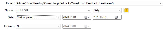
Figure 5: Backtesting our trading application over 5 years of historical EUR/USD market data

To make the test more realistic, we also introduce random delays, since real-life market conditions are unpredictable and delays help simulate that uncertainty.

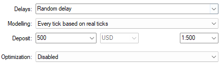
Figure 6: Selecting realistic backtest conditions for our analysis

From there, we can generate a detailed performance summary of our application. In the introduction of this article, I already presented a high-level overview of the backtest results. Here, we see that the system’s Sharpe ratio is low, sitting at 0.34, and the average losing trade is larger than the average winning trade. For fairness, even in our improved version of the application, losing trades still averaged slightly larger than winning trades. However, our closed-loop feedback system managed to reduce this disparity.

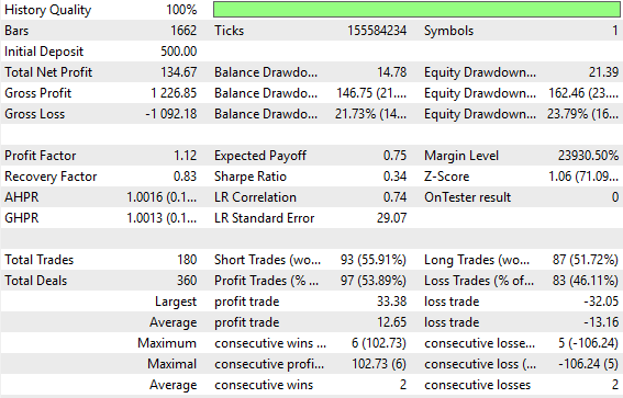
Figure 7: Detailed statistics summarising the performance of our trading application

Additionally, when we examine the equity curve of our baseline system, we see that it does indeed have an upward trend. However, it lacks consistency, often staying range-bound for months at a time—profiting and losing in cycles, essentially leaving the strategy stuck in one place for extended periods. This inconsistency is precisely the behavior we aim to correct by applying our feedback controller to modify the system’s behavior.

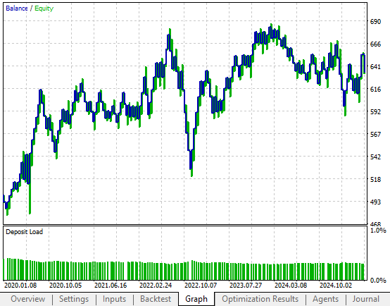
Figure 8: The equity curve produced by our trading application is not satisfactory due to its unstable shape

Improving Our Initial Results

We are now ready to begin improving our initial results using the feedback controller. To avoid unnecessary duplication, I have omitted parts of the code that remain unchanged and will focus mostly on the modifications made to the initial version of our application.

As you can quickly observe, the number of system definitions required for our application has grown. Our initial application needed only one system definition, but the updated version depends on four. These new definitions are tied to: (1) the total number of observations we want to collect before the feedback controller goes online, (2) the number of features we want to keep track of—in this example, twelve features that capture the performance of our trading strategy—and (3) a vector that tracks the type of position we currently hold.

//+------------------------------------------------------------------+
//|                                         Closed Loop Feedback.mq5 |
//|                                               Gamuchirai Ndawana |
//|                    https://www.mql5.com/en/users/gamuchiraindawa |
//+------------------------------------------------------------------+
#property copyright "Gamuchirai Ndawana"
#property link      "https://www.mql5.com/en/users/gamuchiraindawa"
#property version   "1.00"

//+------------------------------------------------------------------+
//| System definitions                                               |
//+------------------------------------------------------------------+
#define MA_PERIOD    10
#define OBSERVATIONS 90
#define FEATURES     12
#define ACCOUNT_STATES 3

The global variables also grow in complexity as our application expands. We now need matrices to store snapshots, vectors to record predictions from our linear system, and Boolean flags to determine when the system is ready to transition from observation to live trading.

//+------------------------------------------------------------------+
//| Global variables                                                 |
//+------------------------------------------------------------------+
int    ma_h_handler,ma_l_handler,atr_handler,scenes,b_matrix_scenes;
double ma_h[],ma_l[],atr[];
matrix snapshots,OB_SIGMA,OB_VT,OB_U,b_vector,b_matrix;
vector S,prediction;
vector account_state;
bool predict,permission;

During initialization, several preprocessing steps are performed. The first few steps are familiar, where we set up our technical indicators. After that, we initialize the snapshot matrix with 12 rows and 90 columns. At this stage, all entries are set to zero. The “permission” flag is initialized as true, meaning the system begins with permission to trade. However, once the 90-day observation period is complete, this flag is set to false, and the “predict” flag is set to true. At that point, the system no longer trades unconditionally; it must first obtain authorization from the linear model before taking action.

//+------------------------------------------------------------------+
//| Expert initialization function                                   |
//+------------------------------------------------------------------+
int OnInit()
  {
//---
   DailyTimeHandler  = new Time(Symbol(),PERIOD_D1);
   TradeInfoHandler  = new TradeInfo(Symbol(),PERIOD_D1);
   ma_h_handler      = iMA(Symbol(),PERIOD_D1,MA_PERIOD,0,MODE_EMA,PRICE_HIGH);
   ma_l_handler      = iMA(Symbol(),PERIOD_D1,MA_PERIOD,0,MODE_EMA,PRICE_LOW);
   atr_handler       = iATR(Symbol(),PERIOD_D1,14);
   snapshots         = matrix::Ones(FEATURES,OBSERVATIONS);
   scenes            = 0;
   b_matrix_scenes   = 0;
   account_state     = vector::Zeros(3);
   b_matrix          = matrix::Zeros(1,1);
   prediction        = vector::Zeros(2);
   predict           = false;
   permission        = true;
//---
   return(INIT_SUCCEEDED);
  }

The OnTick handler has undergone significant changes since the baseline system. A key adjustment is that the account state is now stored in a vector of three entries. This vector uses a one-hot encoding approach: if a buy position is open, the first entry is set to 1; if a sell position is open, the second entry is set to 1; if no position is open, the third entry is set to 1. This provides categorical information to the linear system in a structured format.

The trading logic itself remains the same—if the closing price is above the high of the moving average channel, we consider buying; if it is below the low, we consider selling. During the first 90 days, while the predict flag is false, the system has unconditional permission to trade. Afterward, all trade decisions require validation from the linear system. Once the required number of observations is collected, the snapshot matrix is resized to accommodate new data, and the linear system we have identified filters our trading decisions before we go to the market. 

//+------------------------------------------------------------------+
//| Expert tick function                                             |
//+------------------------------------------------------------------+
void OnTick()
  {
//---
   if(DailyTimeHandler.NewCandle())
     {
      CopyBuffer(ma_h_handler,0,0,1,ma_h);
      CopyBuffer(ma_l_handler,0,0,1,ma_l);
      CopyBuffer(atr_handler,0,0,1,atr);
      double c = iClose(Symbol(),PERIOD_D1,0);

      if(PositionsTotal() == 0)
        {
         account_state = vector::Zeros(ACCOUNT_STATES);

         if(c > ma_h[0])
           {
            if(!predict)
              {
               if(permission)
                  Trade.Buy(TradeInfoHandler.MinVolume(),Symbol(),TradeInfoHandler.GetAsk(),(TradeInfoHandler.GetBid()-(atr[0]*2)),(TradeInfoHandler.GetBid()+(atr[0]*2)),"");
              }

            account_state[0] = 1;
           }

         else
            if(c < ma_l[0])
              {
               if(!predict)
                 {
                  if(permission)
                     Trade.Sell(TradeInfoHandler.MinVolume(),Symbol(),TradeInfoHandler.GetBid(),(TradeInfoHandler.GetAsk()+(atr[0]*2)),(TradeInfoHandler.GetAsk()-(atr[0]*2)),"");
                 }

               account_state[1] = 1;
              }

            else
              {
               account_state[2] = 1;
              }
        }

      if(scenes < OBSERVATIONS)
        {
         take_snapshots();
        }

      else
        {
         matrix temp;
         temp.Assign(snapshots);
         snapshots = matrix::Ones(FEATURES,scenes+1);

         //--- The first row is the intercept and must be full of ones
         for(int i=0;i<FEATURES;i++)
            snapshots.Row(temp.Row(i),i);

         take_snapshots();
         fit_snapshots();

         predict = true;
         permission = false;
        }
      scenes++;
     }
  }

At this stage, the system captures the full snapshot of relevant features: yesterday’s open, high, low, and close prices, the state of technical indicators, account information, and the one-hot encoded account state vector. By including these variables, the system can learn to model our strategy's relationship with the market. Our interests have now out grown simply predicting future price levels, we want to predict the future balance of our trading account. And hopefully, if this relationship exists and can be learned, then our feedback-controller will learn to modfiy the strategy's behavior without human intervention.

//+------------------------------------------------------------------+
//| Record the current state of our system                           |
//+------------------------------------------------------------------+
void take_snapshots(void)
  {
   snapshots[1,scenes] = iOpen(Symbol(),PERIOD_D1,1);
   snapshots[2,scenes] = iHigh(Symbol(),PERIOD_D1,1);
   snapshots[3,scenes] = iLow(Symbol(),PERIOD_D1,1);
   snapshots[4,scenes] = iClose(Symbol(),PERIOD_D1,1);
   snapshots[5,scenes] = AccountInfoDouble(ACCOUNT_BALANCE);
   snapshots[6,scenes] = AccountInfoDouble(ACCOUNT_EQUITY);
   snapshots[7,scenes] = ma_h[0];
   snapshots[8,scenes] = ma_l[0];
   snapshots[9,scenes] = account_state[0];
   snapshots[10,scenes] = account_state[1];
   snapshots[11,scenes] = account_state[2];
  }
//+------------------------------------------------------------------+

We then fit a linear system using two matrices: X for inputs and y for targets. This is a multi-output system, predicting multiple outcomes simultaneously. The y matrix is offset by one time step so that inputs correspond to the previous 89 snapshots and outputs to the subsequent 89 snapshots. As more observations are collected, this loop naturally adapts to the growing dataset by keeping track of the total scenes that have elapsed.

A scene is the time between two subsequent snapshots. In our discussion we collect snapshots of the system everyday, therefore the number of scenes can also be adjusted to fit the reader's preference. Using the pseudo-inverse solution (the PInv() function in MQL5), we solve for the optimal coefficients mapping X to y. This function has been explained in detail in earlier articles in our series. However, any readers unfamiliar with the importance of the role played by the PInv function may consider referring to the discussion linked here, as the PInv() function it is a powerful tool we use.

Once fitted, the system outputs the snapshots, the inputs and targets, the learned coefficients, and its predictions. We then interpret these predictions in real time. If the model anticipates account balance growth, permission to trade is granted. If the model predicts upward momentum in the moving average high while a buy position is under consideration, permission is also granted. Similarly, if the model predicts downward momentum in the moving average low and a sell position is considered, permission is granted. In all other cases, the system withholds permission.

Finally, if permission is granted and no positions are open, the system executes the desired trade. After completing this procedure, the program prints the current balance, the predicted balance, and whether permission was granted. This completes the modifications necessary to start seeing changes in our strategy's performance. The code that we have written does not explicitly instruct the controller when to buy or sell, but the rather, we define for the controller a set actions it can perform, based on deductions it draws, from observations it accumulated.

//+------------------------------------------------------------------+
//| Fit our linear model to our collected snapshots                  |
//+------------------------------------------------------------------+
void fit_snapshots(void)
  {
   matrix X,y;
   X.Reshape(FEATURES,scenes);
   y.Reshape(FEATURES-1,scenes);

   for(int i=0;i<scenes;i++)
     {
      X[0,i] = snapshots[0,i];
      X[1,i] = snapshots[1,i];
      X[2,i] = snapshots[2,i];
      X[3,i] = snapshots[3,i];
      X[4,i] = snapshots[4,i];
      X[5,i] = snapshots[5,i];
      X[6,i] = snapshots[6,i];
      X[7,i] = snapshots[7,i];
      X[8,i] = snapshots[8,i];
      X[9,i] = snapshots[9,i];
      X[10,i] = snapshots[10,i];
      X[11,i] = snapshots[11,i];

      y[0,i] = snapshots[1,i+1];
      y[1,i] = snapshots[2,i+1];
      y[2,i] = snapshots[3,i+1];
      y[3,i] = snapshots[4,i+1];
      y[4,i] = snapshots[5,i+1];
      y[5,i] = snapshots[6,i+1];
      y[6,i] = snapshots[7,i+1];
      y[7,i] = snapshots[8,i+1];
      y[8,i] = snapshots[9,i+1];
      y[9,i] = snapshots[10,i+1];
      y[10,i] = snapshots[11,i+1];
     }

//--- Find optimal solutions
   b_vector = y.MatMul(X.PInv());
   Print("Day Number: ",scenes+1);
   Print("Snapshot");
   Print(snapshots);
   Print("Input");
   Print(X);
   Print("Target");
   Print(y);
   Print("Coefficients");
   Print(b_vector);
   Print("Prediciton");
   Print(y.Col(scenes-1));
   prediction = b_vector.MatMul(snapshots.Col(scenes-1));

   if(prediction[4] > AccountInfoDouble(ACCOUNT_BALANCE))
      permission = true;

   else
      if((account_state[0] == 1) && (prediction[6] > ma_h[0]))
         permission = true;

      else
         if((account_state[1] == 1) && (prediction[7] < ma_l[0]))
            permission = true;

         else
            permission = false;

   if(permission)
     {
      if(PositionsTotal() == 0)
        {
         if(account_state[0] == 1)
            Trade.Buy(TradeInfoHandler.MinVolume(),Symbol(),TradeInfoHandler.GetAsk(),(TradeInfoHandler.GetBid()-(atr[0]*2)),(TradeInfoHandler.GetBid()+(atr[0]*2)),"");

         else
            if(account_state[1] == 1)
               Trade.Sell(TradeInfoHandler.MinVolume(),Symbol(),TradeInfoHandler.GetBid(),(TradeInfoHandler.GetAsk()+(atr[0]*2)),(TradeInfoHandler.GetAsk()-(atr[0]*2)),"");
        }
     }

   Print("Current Balabnce: ",AccountInfoDouble(ACCOUNT_BALANCE)," Predicted Balance: ",prediction[4]," Permission: ",permission);
  }
//+------------------------------------------------------------------+

With this framework complete, we are now ready to backtest our application under the same historical conditions as before. To avoid redundancy, I will not restate the test parameters here, but note that they are identical to those used in Figure 6. 

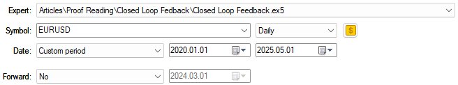
Figure 9: Preparing to test the improved version of our trading strategy

The detailed analysis reveals a stark difference between the baseline and the feedback-controlled system. Net profit has grown substantially, while gross profit remains nearly unchanged—showing that the controller is directly targeting losing trades with some meritable skill. The Sharpe ratio has risen meaningfully, and the average size of profitable and losing trades are now nearly equal, a remarkable improvement over the baseline. 

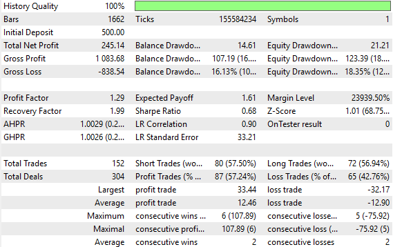
Figure 10: A detailed analysis of the results produced by our trading application shows the improvements we have made

The equity curve shows reduced volatility and a stronger, more consistent upward trend. This is the desired outcome we hoped to observe by implementing a closed-loop fedback controler into our trading strategy.

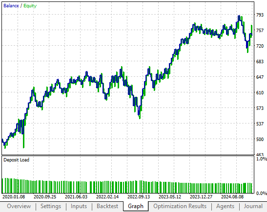
Figure 11: The equity curve produced by our revised trading strategy displays less volatility over time and more stable returns.

I have also attached a screenshot of the snapshots our system was taking during the backtest. Unfortunately, not all 12 features managed to fit into our single screenshot. However, the reader can see that the last row of the snapshot matrix contains the same $500 balance our simulated trading strategy started with, reffer to Figure 6. Then we keep track of how the equity and the balance in our account is being affected by the market conditions and our trading strategy's decision making process.

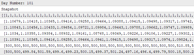
Figure 12: The snapshots of our system's performance that we are keeping track of to monitor and correct our strategy

A journal snapshot of the outputs confirms this behavior. For example, on day 1645, the permission flag was set to false because the linear system expected a loss and blocked the trade. 

Figure 13: Our linear system controller denied our trading strategy permission to trade because it analysed unfavourable market conditions

The very next day, when profitability was expected, the system granted permission and executed the trade. All in all, this is how the improved application operates from start to finish. This shows that there are many use cases for predictive models beyond ordinary price prediction. We can employ these learned models to test if there exists any structure we can learn from that dominates our winning and loosing trades. To help us learn to refrain from repeating past mistakes.

Figure 14: When market conditions appear to be aligned with our strategy, our feedback controller give us permission to continue trading

Conclusion

In conclusion, feedback controllers give us a way to build trading systems that are not only profitable but also adaptive. By learning from their own performance, these systems may help us avoid repeating past mistakes and remain effective even in changing market conditions. Our results show clear improvements in profitability, efficiency, and risk reduction, proving that control theory has real practical value in trading. Looking forward, this work motivates us to expand beyond linear models and explore nonlinear feedback controllers that may capture even richer patterns in market behavior. With these advances, we can continue to push our systems toward greater stability and profitability in the face of uncertainty.

However, before we look past our linear system, there are still valuable improvements we can make. Measuring the value of each of these possible improvements on a simple linear systems will give us a reliable benchmark for any other non-linear system we may want to build.