Reimagining Classic Strategies (Part 15): Daily Breakout Trading Strategy

In this series of articles, we often seek to employ machine learning models to help improve the performance of our trading strategies. However, we often overlook the fact that these models make many blind assumptions about the data at hand. Furthermore, classical statistical learning does not offer us any guidance in proving whether the relationships we are trying to model actually exist in reality.

Human traders, on the other hand, have learned over many years of interaction with the markets a certain fundamental essence of what we may call market logic. This insight, which we will refer to as market logic, is gained only from experience. Hopefully, we can integrate the findings that these human traders have learned into our numerically driven trading applications. Discretionary traders have been active in financial markets long before the existence of computers. Therefore, there may be some meritable truth in the rules of thumb they have learned to value over the years—rules that we may be able to employ.

As we have already stated, we typically use machine learning algorithms to help us learn relationships that project the past onto the future. However, we almost always assume such a relationship exists and can be learned from the data. We rarely take the time to prove that these relationships exist in the first place. Discretionary traders, by necessity, have essentially been forced to look for reliable relationships that could sustain their careers. From this perspective, we could argue that human traders were forced to do the manual labor that can set the foundation for our machine learning models to build on.

We therefore seek to bridge the gap between machine learning and financial trading by using the heuristics and rules of thumb that human beings have developed over many years of interaction with the markets. These rules, which traders have generally learned to abide by, may serve as a framework that enables our models to learn financial markets in a more structured way. Instead of having our models prove relationships from scratch, we can extend principles that have already been proven valid over time. This gives our models a head start rather than asking them to begin at rest.

The most important part of our test is proving the validity of the strategy we begin with. For this reason, our trading strategy was based on a well-known breakout approach that relies on the relationship between consecutive trading days. The strategy in essence is rather simple.

Overview of Our Trading Strategy

On the beginning each trading day, we begin by marking the prior day’s high and low.

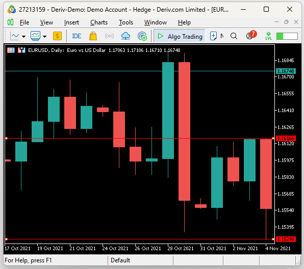
Figure 1: Setting up our daily breakout strategy by marking the previous day high and low price levels

When the price breaks the prior day’s high, we enter a short position and take profits at the prior day’s low. Conversely, when the price breaks the prior day’s low, we enter a long position and take profits at the prior day’s high. It is essentially a contrarian trading strategy, looking for one breakout trade each day.

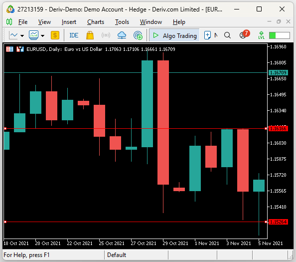
Figure 2: Our entry signals are triggered the first time price levels breach the previous day extreme level

Interestingly, even without predictive modeling or advanced neural networks, we observed that a sound understanding of how financial markets work is an invaluable asset. In its original form, as primitive as it may appear, this daily breakout strategy achieved accuracy levels that rivaled the performance of a deep neural network—simply by relying on market logic learned by discretionary traders.

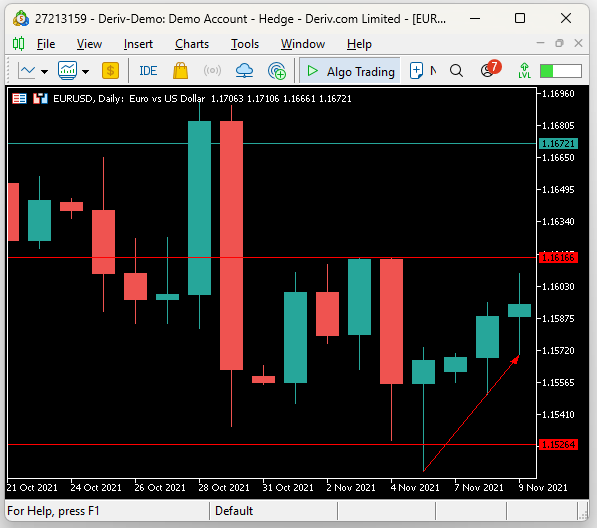
Figure 3: The strategy exists its positions when the opposite extreme price level is breached, but as we can see in the illustration above, the strategy contains some amount of error

We also observed that the strategy was overly aggressive and unstable. The exiting rules defined by the strategy are not always satisfied completely, as illustrated by Figure 3. Therefore, modifications were necessary to exercise some level of control over its volatility. The volatility I refer to here is the fluctuating behavior of profit in the account during the backtest.

As we will see in the subsequent sections, we first implemented the original trading strategy in its simplest form—true to the description accepted by most traders—to establish a baseline performance level. Afterward, we made modifications to the strategy and compared improvements against the original version to ensure that our changes moved us in the desired direction. The changes we made affected the strategy in three important dimensions:

Profitability

Our original strategy produced a profit of only $40 over a five-year backtest. This is not impressive on any scale. However, what was impressive was that 68% of all trades placed were profitable, which is remarkable for an out-of-sample test across five years—especially since the strategy had no tuning parameters and relied solely on logic and intuition. Unfortunately, the average losing trade tended to be larger than the average winning trade, resulting in that dismal $40 profit.

After several iterations, our improved version of the strategy produced a profit of $162 over the same period—a 300% improvement. In addition, we managed to improve the strategy’s Sharpe ratio from 0.13 to 0.40, a 207% improvement over the original. The reader should note here that all trades were fixed to the minimum lot position allowed, to challenge our application to demonstrate true skill.

Trading Efficiency

The initial strategy required 886 trades in total to realize its dismal $40 profit, while our improved version required only 246 trades to realize $162. This means the improved strategy achieved a 72% reduction in trading activity and unnecessary market exposure, and moreover realized larger returns. This is a coveted feature of any trading application: more gains while taking on less risk.

In the original strategy, the average profit was $3.64 and the average loss was $7.87. We managed to correct this behavior. In our improved version, we achieved an average profit of $14.82 while at the same time keeping the average loss almost at par at $7.95. 

Trading Accuracy

Unfortunately, while these changes improved profitability and efficiency, they negatively affected our accuracy. The proportion of winning trades fell from 68% in the original strategy to 37% in the improved version—a 45% reduction in accuracy. The original strategy’s high accuracy rate had been one of its most appealing features, and attempts to manually fine-tune without sacrificing accuracy proved difficult.

Therefore, we may consider giving this task instead to a feedback controller, as demonstrated in our previous discussion (link provided here). We also believe it would be valuable to continue testing more discretionary trading rules that human traders have relied on for years, selectively filtering out those that naturally produce high accuracy levels, such as the results we began with. In doing so, these strategies may offer a structured framework for our machine learning models to learn both the strengths and the limitations of human intuition. Let us get started.

Getting Started in MQL5

As with most of our applications, we will begin by defining the necessary global variables to follow the strategy. We'll need identifiers for the two price levels we keep track of, the previous day's high and low. We'll also mark these price levels with horizontal lines running across our chart, therefore we'll need strings to store the names of our price levels.

//+------------------------------------------------------------------+
//|                                                         UB 2.mq5 |
//|                                               Gamuchirai Ndawana |
//|                    https://www.mql5.com/en/users/gamuchiraindawa |
//+------------------------------------------------------------------+
#property copyright "Gamuchirai Ndawana"
#property link      "https://www.mql5.com/en/users/gamuchiraindawa"
#property version   "1.00"

//+------------------------------------------------------------------+
//| Global Variables                                                 |
//+------------------------------------------------------------------+
double last_high,last_low;
string h,l;
bool rest;
int atr_handler;
double atr[];

Likewise, we'll import the trade library to help us manage our positions during backtesting.

//+------------------------------------------------------------------+
//| Libraries                                                        |
//+------------------------------------------------------------------+
#include <Trade\Trade.mqh>
CTrade Trade;

When our application is loaded for the first time, we'll store the names of the two price levels we are tracking, set up the Average True Range (ATR) indicator for our risk management, and lastly, we'll reset a system flag named "rest." As the name implies, our system will look for trades until rest is set to true. At that point, the system will stop searching for setups, and instead manage the open positions.

//+------------------------------------------------------------------+
//| Expert initialization function                                   |
//+------------------------------------------------------------------+
int OnInit()
  {
//---
   h="high";
   l="low";
   rest = false;
   atr_handler = iATR(Symbol(),PERIOD_H8,4*14);
//---
   return(INIT_SUCCEEDED);
  }

When our application is no longer in use, we'll release the ATR indicator to clean up after ourselves and share the memory with the rest of the system. 

//+------------------------------------------------------------------+
//| Expert deinitialization function                                 |
//+------------------------------------------------------------------+
void OnDeinit(const int reason)
  {
//---
   IndicatorRelease(atr_handler);
  }

Once, at the beginning of each day, we will store the highest and lowest price levels that were offered the day before.

//---
   datetime cd = iTime(Symbol(),PERIOD_D1,0);
   static datetime ds;

   if(cd != ds)
     {
      ds = cd;
      last_high = iHigh(Symbol(),PERIOD_D1,1);
      last_low = iLow(Symbol(),PERIOD_D1,1);

      if((rest==true) && (PositionsTotal() == 0))
         rest = false;

      Comment("Last High: ",last_high,"\nLast Low: ",last_low);

      ObjectDelete(0,l);
      ObjectDelete(0,h);

      ObjectCreate(0,h,OBJ_HLINE,0,0,last_high);
      ObjectCreate(0,l,OBJ_HLINE,0,0,last_low);
      CopyBuffer(atr_handler,0,0,1,atr);
     }

As the day progresses, we will enter contrarian positions when the first extreme price level is broken, this first break is believed to be the true trend for that day.

   datetime ch = iTime(Symbol(),PERIOD_H1,0);
   static datetime hs;

   if(ch != hs)
     {
      hs = ch;
      double bid,ask,close,padding;

      close = iClose(Symbol(),PERIOD_H1,0);
      ask = SymbolInfoDouble(Symbol(),SYMBOL_ASK);
      bid = SymbolInfoDouble(Symbol(),SYMBOL_BID);
      padding = atr[0] * 2;

      if(rest == false)
        {
         if(PositionsTotal() == 0)
           {

            if(close<last_low)
               Trade.Buy(0.01,Symbol(),ask,(bid-(padding)),last_high);
               
            else
               if(close>last_high)
                  Trade.Sell(0.01,Symbol(),bid,(ask+(padding)),last_low);
                  
            rest = true;
           }
        }
     }
  }
//+------------------------------------------------------------------+

The strategy is mostly based on intuition, and therefore it has few moving parts. We have completed the setup necessary for our application, and we can now start backtesting the trading application.

We begin by selecting five years of historical EUR/USD data in order to see how our application will perform.  

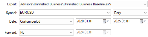
Figure 4: Establishing a baseline performance level using the original version of our trading strategy

Afterward, we set our delay settings to use random delays to simulate the unpredictability of real-life trading.

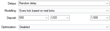
Figure 5: Using random delay settings ensures that you will obtain reliable simulation settings

When we plot the account equity over time, we can see that the strategy—though rather naïve and simple—does produce a positive trend in equity. However, the peaks and valleys it creates are far too wide apart, and we need measures to make the strategy less aggressive and more controlled.

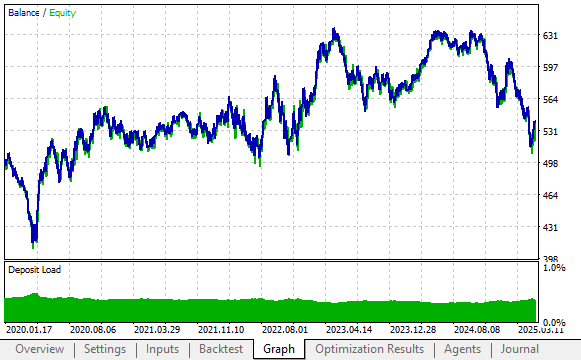
Figure 6: The equity curve produced by the original version of our trading strategy lacks consistency and appears too volatile

Still, the total profit realized by the strategy in its original form was only forty dollars from five years of backtesting. What is impressive, though, is the remarkably high accuracy rate: 68% of all trades placed by the strategy were profitable. The problem, however, was that our average winning trade was smaller than our average losing trade—losses were nearly twice as large

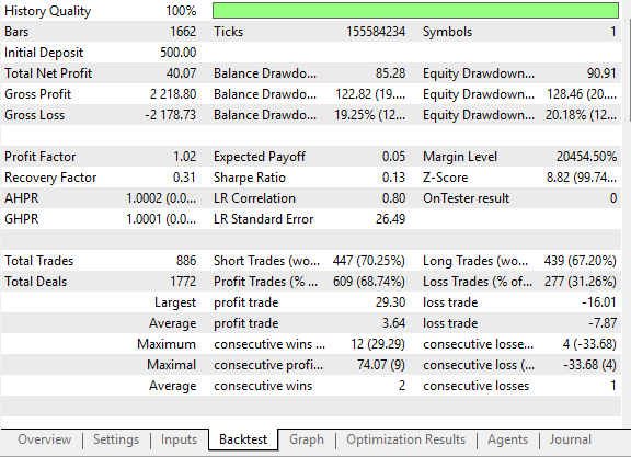
Figure 7: The detailed statistics of our original strategy are remarkable for their naturally high percentage of profitable trades

Making Improvements

Therefore, to improve the original strategy, we had to think creatively about how the strategy analyzes the market, and whether there are ways to anticipate moves without having to wait the entire day for a price level to be broken. After much consideration, I realized that during the first hour of each day, we could compare the gap between the opening price of the day and the previous day’s extreme points.

This gives us the size of the gap between yesterday’s high and low, and the new opening. Our intuition is that price will tend to move in the direction of the larger gap. Therefore: If the day starts closer to its previous low, we go long. Conversely, if the day starts closer to its previous high, we go short.

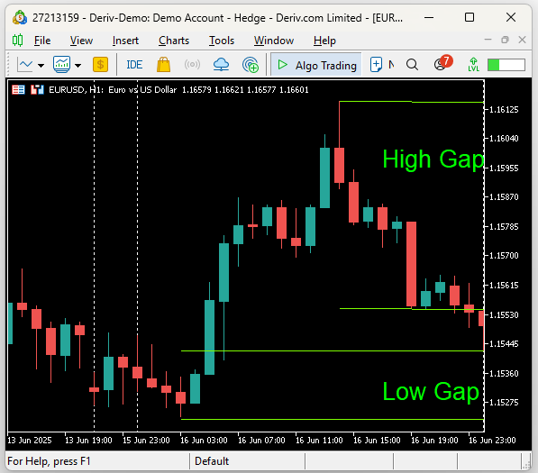
Figure 8: Visualizing improvements we can make to the original version of our trading strategy

Implementing this improvement increased our total net profit from the original forty dollars. This allowed us to anticipate each day’s move without waiting for the traditional rules of the strategy. Only slight modifications were needed in our entry rules: we now considered the absolute value of the gap between the current close and the previous high and low. If the gap to the high was larger, we entered long positions. Otherwise, we entered short positions. After entering each position, the reset parameter was set, and then we will only look for new trades only if the trade was completed.

      if(rest == false)
        {
         if(PositionsTotal() == 0)
           {
            //High Gap Is Bigger
            if(MathAbs(close - last_high) > MathAbs(close - last_low))
               Trade.Buy(0.01,Symbol(),ask,(bid-(padding)),last_high);
	       rest = true;

            
            //Low Gap Is Bigger
            else
               if(MathAbs(close - last_high) < MathAbs(close - last_low))
                  Trade.Sell(0.01,Symbol(),bid,(ask+(padding)),last_low);
	          rest = true;
           }
        }

When combined, our new application looked like this:

//+------------------------------------------------------------------+
//|                                                         UB 2.mq5 |
//|                                               Gamuchirai Ndawana |
//|                    https://www.mql5.com/en/users/gamuchiraindawa |
//+------------------------------------------------------------------+
#property copyright "Gamuchirai Ndawana"
#property link      "https://www.mql5.com/en/users/gamuchiraindawa"
#property version   "1.00"

//+------------------------------------------------------------------+
//| Global Variables                                                 |
//+------------------------------------------------------------------+
double last_high,last_low;
string h,l;
bool rest;
int atr_handler;
double atr[];

//+------------------------------------------------------------------+
//| Libraries                                                        |
//+------------------------------------------------------------------+
#include <Trade\Trade.mqh>
CTrade Trade;

//+------------------------------------------------------------------+
//| Expert initialization function                                   |
//+------------------------------------------------------------------+
int OnInit()
  {
//---
   h="high";
   l="low";
   rest = false;
   atr_handler = iATR(Symbol(),PERIOD_H8,4*14);
//---
   return(INIT_SUCCEEDED);
  }
//+------------------------------------------------------------------+
//| Expert deinitialization function                                 |
//+------------------------------------------------------------------+
void OnDeinit(const int reason)
  {
//---
   IndicatorRelease(atr_handler);
  }
//+------------------------------------------------------------------+
//| Expert tick function                                             |
//+------------------------------------------------------------------+
void OnTick()
  {
//---
   datetime cd = iTime(Symbol(),PERIOD_D1,0);
   static datetime ds;

   if(cd != ds)
     {
      ds = cd;
      last_high = iHigh(Symbol(),PERIOD_D1,1);
      last_low = iLow(Symbol(),PERIOD_D1,1);

      if((rest==true) && (PositionsTotal() == 0))
         rest = false;


      Comment("Last High: ",last_high,"\nLast Low: ",last_low);

      ObjectDelete(0,l);
      ObjectDelete(0,h);

      ObjectCreate(0,h,OBJ_HLINE,0,0,last_high);
      ObjectCreate(0,l,OBJ_HLINE,0,0,last_low);
      CopyBuffer(atr_handler,0,0,1,atr);
     }

   datetime ch = iTime(Symbol(),PERIOD_H1,0);
   static datetime hs;

   if(ch != hs)
     {
      hs = ch;
      last_high = iHigh(Symbol(),PERIOD_D1,1);
      last_low = iLow(Symbol(),PERIOD_D1,1);
      double bid,ask,close,padding;

      close = iClose(Symbol(),PERIOD_H1,0);
      ask = SymbolInfoDouble(Symbol(),SYMBOL_ASK);
      bid = SymbolInfoDouble(Symbol(),SYMBOL_BID);
      padding = atr[0] * 2;

      if(rest == false)
        {
         if(PositionsTotal() == 0)
           {
            if(MathAbs(close - last_high) > MathAbs(close - last_low))
               Trade.Buy(0.01,Symbol(),ask,(bid-(padding)),last_high);

            else
               if(MathAbs(close - last_high) < MathAbs(close - last_low))
                  Trade.Sell(0.01,Symbol(),bid,(ask+(padding)),last_low);

            rest = true;
           }
        }
     }
  }
//+------------------------------------------------------------------+

The equity curve produced by our improved strategy reached new highs that were not achieved by the original version. Our total net profit rose to 148 dollars from the original 40. However, we could already see that the proportion of winning trades was starting to decline.

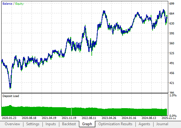
Figure 9: Visualizing the equity curve produced by our new and improved version of the original trading strategy

On one hand, our efficiency improved because we realized $108 more in profits. But, while the original strategy required 886 trades to realize $40, our new version required only 469 trades to realize $148. The strategy is clearly moving in the right direction, but further refinements are still possible.

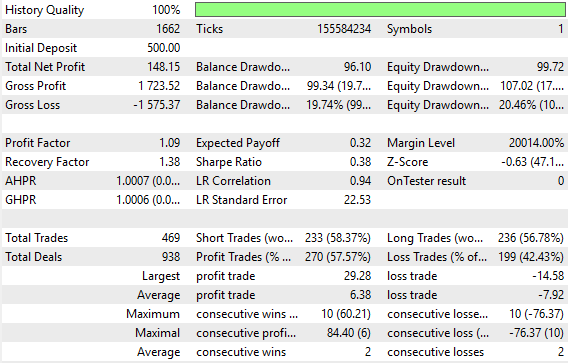
Figure 10: A statistical analysis of the improvements we have made over the original version of the strategy

Making Additional Improvements

To explore this, let us consider the diagram below. We illustrate the high gap as the green rectangle and the low gap as the blue rectangle. Our working theory so far is that price moves in the direction of the larger gap. Currently, we take profits once price breaches the previous day’s extreme point. 

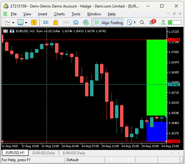
Figure 11: The green and blue rectangles represents yesterday's high and low gaps respectively

However, as we can see, price does not always fully break past these extremes—sometimes it comes close but fails to cross.

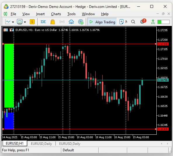
Figure 12: The exit conditions of the original strategy are not consistently satisfied by all possible market conditions

Therefore, we might reason that instead of placing our take profits above the previous extreme, we should place them just beneath it—perhaps a fraction of the ATR below the previous high. That way, as long as price comes close enough, we still capture profits.

Additionally, we want to pull our stop losses tighter as trades move in our favor, to capture as much profit as possible. To implement this, we modified our rules: instead of adding equal padding to stop loss and take profit, we now add a smaller fraction to take profit than to stop loss. This makes the stop loss more forgiving while keeping the take profit tighter to capture momentum.

While positions are open, we also conditionally check if a new stop loss suggestion is more favorable than the current one. Ideally, we always want our stop loss bound to the last extreme price when possible.

   if(ch != hs)
     {
      hs = ch;
      last_high = iHigh(Symbol(),PERIOD_D1,1);
      last_low = iLow(Symbol(),PERIOD_D1,1);
      double bid,ask,close,padding;

      close = iClose(Symbol(),PERIOD_H1,0);
      ask = SymbolInfoDouble(Symbol(),SYMBOL_ASK);
      bid = SymbolInfoDouble(Symbol(),SYMBOL_BID);
      padding = atr[0] * 2;

      if(rest == false)
        {
         if(PositionsTotal() == 0)
           {

            if((MathAbs(close - last_high) > MathAbs(close - last_low)))
               Trade.Buy(0.01,Symbol(),ask,(bid-(padding)),last_high+(padding*0.9));

            else
               if((MathAbs(close - last_high) < MathAbs(close - last_low)))
                  Trade.Sell(0.01,Symbol(),bid,(ask+(padding)),last_low-(padding*0.9));

            rest = true;
           }
        }

      if(rest == true)
        {
         if(PositionsTotal() > 0)
           {
            if(PositionSelectByTicket(PositionGetTicket(0)))
              {
               double sl,tp;

               sl = PositionGetDouble(POSITION_SL);
               tp = PositionGetDouble(POSITION_TP);

               //--- Buy
               if(sl < tp)
                 {
                  if(last_low > sl)
                     Trade.PositionModify(Symbol(),last_low,tp);
                 }

               if(tp < sl)
                 {
                  if(last_high < sl)
                     Trade.PositionModify(Symbol(),last_high,tp);
                 }
              }
           }
        }
     }

When put together, this gave us the final version of the application so far:

//+------------------------------------------------------------------+
//|                                                         UB 2.mq5 |
//|                                               Gamuchirai Ndawana |
//|                    https://www.mql5.com/en/users/gamuchiraindawa |
//+------------------------------------------------------------------+
#property copyright "Gamuchirai Ndawana"
#property link      "https://www.mql5.com/en/users/gamuchiraindawa"
#property version   "1.00"

//+------------------------------------------------------------------+
//| Global Variables                                                 |
//+------------------------------------------------------------------+
double last_high,last_low;
string h,l;
bool rest;
int atr_handler;
double atr[];

//+------------------------------------------------------------------+
//| Libraries                                                        |
//+------------------------------------------------------------------+
#include <Trade\Trade.mqh>
CTrade Trade;

//+------------------------------------------------------------------+
//| Expert initialization function                                   |
//+------------------------------------------------------------------+
int OnInit()
  {
//---
   h="high";
   l="low";
   rest = false;
   atr_handler = iATR(Symbol(),PERIOD_H8,4*14);
//---
   return(INIT_SUCCEEDED);
  }
//+------------------------------------------------------------------+
//| Expert deinitialization function                                 |
//+------------------------------------------------------------------+
void OnDeinit(const int reason)
  {
//---
      IndicatorRelease(atr_handler);
  }
//+------------------------------------------------------------------+
//| Expert tick function                                             |
//+------------------------------------------------------------------+
void OnTick()
  {
//---
   datetime cd = iTime(Symbol(),PERIOD_D1,0);
   static datetime ds;

   if(cd != ds)
     {
      ds = cd;
      last_high = iHigh(Symbol(),PERIOD_D1,1);
      last_low = iLow(Symbol(),PERIOD_D1,1);

      if((rest==true) && (PositionsTotal() == 0))
         rest = false;

      Comment("Last High: ",last_high,"\nLast Low: ",last_low);

      ObjectDelete(0,l);
      ObjectDelete(0,h);

      ObjectCreate(0,h,OBJ_HLINE,0,0,last_high);
      ObjectCreate(0,l,OBJ_HLINE,0,0,last_low);
      CopyBuffer(atr_handler,0,0,1,atr);
     }

   datetime ch = iTime(Symbol(),PERIOD_H1,0);
   static datetime hs;

   if(ch != hs)
     {
      hs = ch;
      last_high = iHigh(Symbol(),PERIOD_D1,1);
      last_low = iLow(Symbol(),PERIOD_D1,1);
      double bid,ask,close,padding;

      close = iClose(Symbol(),PERIOD_H1,0);
      ask = SymbolInfoDouble(Symbol(),SYMBOL_ASK);
      bid = SymbolInfoDouble(Symbol(),SYMBOL_BID);
      padding = atr[0] * 2;

      if(rest == false)
        {
         if(PositionsTotal() == 0)
           {

            if((MathAbs(close - last_high) > MathAbs(close - last_low)))
               Trade.Buy(0.01,Symbol(),ask,(bid-(padding)),last_high+(padding*0.9));

            else
               if((MathAbs(close - last_high) < MathAbs(close - last_low)))
                  Trade.Sell(0.01,Symbol(),bid,(ask+(padding)),last_low-(padding*0.9));

            rest = true;
           }
        }

      if(rest == true)
        {
         if(PositionsTotal() > 0)
           {
            if(PositionSelectByTicket(PositionGetTicket(0)))
              {
               double sl,tp;

               sl = PositionGetDouble(POSITION_SL);
               tp = PositionGetDouble(POSITION_TP);

               //--- Buy
               if(sl < tp)
                 {
                  if(last_low > sl)
                     Trade.PositionModify(Symbol(),last_low,tp);
                 }

               if(tp < sl)
                 {
                  if(last_high < sl)
                     Trade.PositionModify(Symbol(),last_high,tp);
                 }
              }
           }
        }
     }
  }

The equity curve now rises to higher levels than either of the earlier strategies. Volatility—the range between wins and losses—is also more controlled.

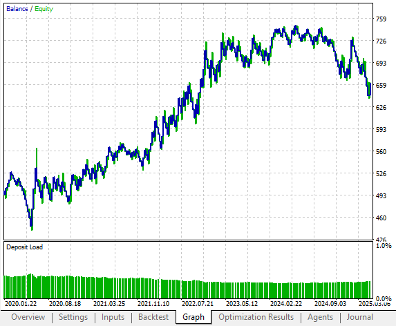
Figure 13: The final version of our trading strategy produced an equity curve with the desired structure we didn't have originally

Looking at the detailed statistics, we see total net profit has again increased, from $148 in the previous version to $162 in this version. However, the proportion of winning trades is again smaller than before, and smaller than in the original strategy as well. This shows that our improvements are not only affecting profitable trades, but also unprofitable ones in ways we do not desire.

This highlights a deeper challenge: improving trading strategies built on human intuition alone is not easy to solve with further intuition. To truly move forward, we must consider other ways of improving beyond human judgment.

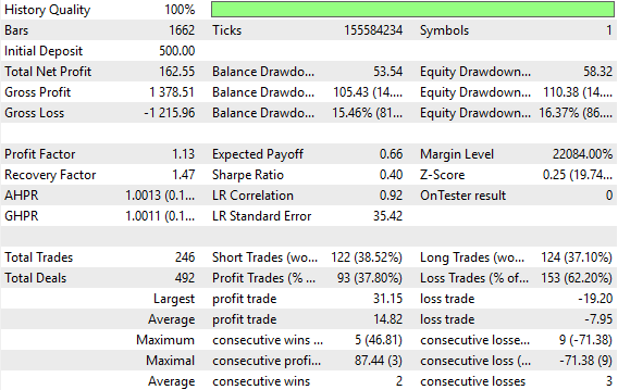
Figure 14: Upon closer inspection, we realised that our modifications also negatively affected the system's performance in terms of accuracy

Conclusion

Human traders did not survive in financial markets by chance or by hacking their way forward one trade at a time. They were forced, by necessity and by the fear of loss, to seek out relationships that were real and reliable. This discipline is often overlooked today, as machine learning practitioners rush toward bigger data and more complex models without questioning whether their metrics truly reflect meaningful progress.

Our work suggests another path. By grounding strategies in discretionary market logic, we begin from a place of demonstrated validity rather than blind assumption. The residuals of these strategies—the error in our strategies—become fertile ground for machine learning models. In this way, we no longer ask our algorithms to prove relationships from scratch; instead, we give them a framework where the inputs and outputs are already connected.

This shift also brings us closer to satisfying the statistical assumptions our models quietly depend on. A fixed strategy facing a changing market generates outputs that resemble the independent, identically distributed conditions required for robust learning. The real world may never be perfectly IID, but this approach edges us closer to that ideal, making our models less fragile and more trustworthy. Our belief is that by starting with market logic learned by humans, and then training models on the error in the logic, we may enable our machine learning models to start learning from higher ground.

File Name	File Details
Daily Breakout Strategy V1.mq5	The initial and aggressive version of our trading strategy that had high initial trading accuracy.
Daily Breakout Strategy V2.mq5	The second version of our trading application that had slightly lower accuracy levels but significantly greater profitability levels.
Daily Breakout Strategy V3.mq5	The final version of our trading strategy that produced the highest profit levels but the lowest accuracy levels.