Integrating MQL5 with data processing packages (Part 5): Adaptive Learning and Flexibility

Introduction

The problem many algorithmic traders face lies in the rigidity and lack of adaptability in traditional trading systems. As discussed in the previous article, most-rule based Expert Advisors (EAs) are hardcoded with static conditions and thresholds, which often fail to adjust to changing market dynamics, volatility shifts, or unseen patterns in real-time. As a result, these systems perform well during specific market regimes but deteriorate in performance when market behavior changes, leading to missed opportunities, frequent false signals, or prolonged drawdowns.

Adaptive learning and flexibility modes provide a compelling solution to this problem. By using Python to build a reinforcement learning model capable of continuously learning from historical XAUUSD price action we enable the system to adjust its strategy based on evolving market conditions. The flexibility of Python libraries (like PyTorch, Gym, Pandas, etc.) allows for advanced data preprocessing, environment simulation, and model optimization. Once trained, the model can be exported to ONNX, enabling deployment within the MQL5 environment.

Getting Historical Data

from datetime import datetime
import MetaTrader5 as mt5
import pandas as pd
import pytz

# Display data on the MetaTrader 5 package
print("MetaTrader5 package author: ", mt5.__author__)
print("MetaTrader5 package version: ", mt5.__version__)

# Configure pandas display options
pd.set_option('display.max_columns', 500)
pd.set_option('display.width', 1500)

# Establish connection to MetaTrader 5 terminal
if not mt5.initialize():
    print("initialize() failed, error code =", mt5.last_error())
    quit()

# Set time zone to UTC
timezone = pytz.timezone("Etc/UTC")
# Create 'datetime' objects in UTC time zone to avoid the implementation of a local time zone offset
utc_from = datetime(2025, 05, 15, tzinfo=timezone.utc)
utc_to = datetime.(2025, 07,08, tzinfo=timezone.utc) 

# Get bars from XAU H1 (hourly timeframe) within the specified interval
rates = mt5.copy_rates_range("XAUUSD", mt5.TIMEFRAME_H1, utc_from, utc_to)

# Shut down connection to the MetaTrader 5 terminal
mt5.shutdown()

# Check if data was retrieved
if rates is None or len(rates) == 0:
    print("No data retrieved. Please check the symbol or date range.")
else:
    # Display each element of obtained data in a new line (for the first 10 entries)
    print("Display obtained data 'as is'")
    for rate in rates[:10]:
        print(rate)

    # Create DataFrame out of the obtained data
    rates_frame = pd.DataFrame(rates)
    # Convert time in seconds into the 'datetime' format
    rates_frame['time'] = pd.to_datetime(rates_frame['time'], unit='s')

    # Save the data to a CSV file
    filename = "XAU_H1.csv"
    rates_frame.to_csv(filename, index=False)
    print(f"\nData saved to file: {filename}")

To retrieve historical data, we begin by initializing a connection to the MetaTrader 5 terminal using the mt5.initialize() function, which enables communication between Python and the MetaTrader 5 platform. We then define the specific date range for data extraction by setting both a start and end date. These dates are handled as datetime objects in UTC to maintain consistency across time zones. In this case, the script is configured to request historical hourly data for the XAUUSD symbol, covering the period from May 15, 2025, to July 8, 2025, using the mt5.copy_rates_range() function.

filename = "XAUUSD_H1.csv"
rates_frame.to_csv(filename, index=False)
print(f"\nData saved to file: {filename}")

As you may know by now my OS is Linux. If your OS is Windows, you can simply get the historical date with the following python script:

from datetime import datetime
import MetaTrader5 as mt5
import pandas as pd
import pytz

# Display data on the MetaTrader 5 package
print("MetaTrader5 package author: ", mt5.__author__)
print("MetaTrader5 package version: ", mt5.__version__)

# Configure pandas display options
pd.set_option('display.max_columns', 500)
pd.set_option('display.width', 1500)

# Establish connection to MetaTrader 5 terminal
if not mt5.initialize():
    print("initialize() failed, error code =", mt5.last_error())
    quit()

# Set time zone to UTC
timezone = pytz.timezone("Etc/UTC")
# Create 'datetime' objects in UTC time zone to avoid the implementation of a local time zone offset
utc_from = datetime(2025, 05, 15, tzinfo=timezone.utc)
utc_to = datetime(2025, 07, 08, tzinfo=timezome.utc) 

# Get bars from XAUUSD H1 (hourly timeframe) within the specified interval
rates = mt5.copy_rates_range("XAUUSD", mt5.TIMEFRAME_H1, utc_from, utc_to)

# Shut down connection to the MetaTrader 5 terminal
mt5.shutdown()

# Check if data was retrieved
if rates is None or len(rates) == 0:
    print("No data retrieved. Please check the symbol or date range.")
else:
    # Display each element of obtained data in a new line (for the first 10 entries)
    print("Display obtained data 'as is'")
    for rate in rates[:10]:
        print(rate)

    # Create DataFrame out of the obtained data
    rates_frame = pd.DataFrame(rates)
    # Convert time in seconds into the 'datetime' format
    rates_frame['time'] = pd.to_datetime(rates_frame['time'], unit='s')

    # Display data directly
    print("\nDisplay dataframe with data")
    print(rates_frame.head(10)

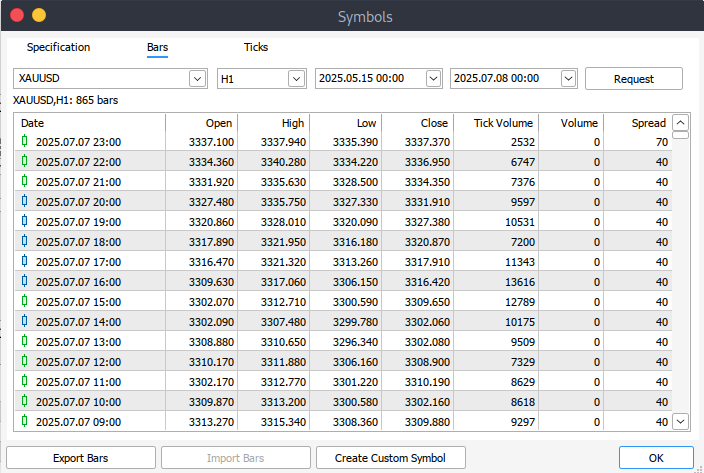
If you're unable to retrieve historical data programmatically, you can manually download it directly from your MetaTrader 5 platform. Start by launching the platform, then go to the top menu and navigate to Tools > Options, which will bring you to the Charts settings. Here, you'll need to specify how many bars to display on the chart. It's recommended to select the "unlimited bars" option, especially since we'll be working with date ranges and can't precisely predict how many bars a given timeframe will contain.

Next, to download the actual data, go to View > Symbols in the menu bar, which opens the Symbols window under the Specifications tab. From there, choose either the Bars or Ticks tab, depending on the type of data you need. Enter the desired start and end dates for your historical data, then click the Request button. Once the data has been retrieved, you can export and save it in .csv format for later use.

Getting started

import pandas as pd

# Load the uploaded BTC 1H CSV file
file_path = '/home/int_j/Documents/Art Draft/Data Science/Adaptive Learning/XAUUSD_H1.csv'
xau_data = pd.read_csv(file_path)

# Display basic information about the dataset
xau_data_info = xau_data.info()
xau_data_head = xau_data.head()

xau_data_info, xau_data_head

We begin by examining the dataset to understand its structure. This involves checking the data types, dimensions, and completeness using the info() function. Additionally, we preview the first few rows with head() to get a sense of the dataset’s content and layout. This step is a standard part of exploratory data analysis, helping confirm the data was imported correctly and providing an initial overview of its format.

# Reload the data with tab-separated values
xau_data = pd.read_csv(file_path, delimiter='\t')

# Display basic information and the first few rows after parsing
xau_data_info = xau_data.info()
xau_data_head = xau_data.head()

xau_data_info, xau_data_head

This code block begins by reloading the XAUUSD historical data from a specified file path, using tab (\t) as the delimiter instead of the default comma. It is important when dealing with TSV (Tab-Separated Values) files to ensure the data is parsed correctly. After loading the data into the xau_data DataFrame, it prints out essential information about the dataset such as column types, non-null counts, and memory usage, using info(), and also shows the first few rows with head() for a quick preview.

import pandas as pd
import numpy as np
import ta
from sklearn.preprocessing import StandardScaler

# Split the single column into proper columns
if len(xau_data.columns) == 1:
    # Extract column headers from the first row
    headers = xau_data.columns[0].split('\t')
    
    # Split data into separate columns
    xau_data = xau_data[xau_data.columns[0]].str.split('\t', expand=True)
    xau_data.columns = headers

# Convert columns to proper data types
numeric_cols = ['<OPEN>', '<HIGH>', '<LOW>', '<CLOSE>', '<TICKVOL>', '<VOL>', '<SPREAD>']
xau_data[numeric_cols] = xau_data[numeric_cols].apply(pd.to_numeric, errors='coerce')

# Clean and create features
xau_data = xau_data.dropna()
xau_data['return'] = xau_data['<CLOSE>'].pct_change()

# Add technical indicators
xau_data['rsi'] = ta.momentum.RSIIndicator(xau_data['<CLOSE>'], window=14).rsi()
xau_data['macd'] = ta.trend.MACD(xau_data['<CLOSE>']).macd_diff()
xau_data['sma_20'] = ta.trend.SMAIndicator(xau_data['<CLOSE>'], window=20).sma_indicator()
xau_data['sma_50'] = ta.trend.SMAIndicator(xau_data['<CLOSE>'], window=50).sma_indicator()
xau_data = xau_data.dropna()

# Normalize features
scaler = StandardScaler()
features = ['rsi', 'macd', 'sma_20', 'sma_50', 'return']
xau_data[features] = scaler.fit_transform(xau_data[features])

Int his code block, the process begins with cleaning and formatting the historical XAUUSD dataset. If the data was incorrectly loaded as a single column (which can happen with tab-separated files), the script splits that column using tabs to extract the proper headers and values. Afterward, it explicitly converts key columns such as open, high, low, close, volume, and spread to numeric data types, handling any errors during conversion with errors='coerce'. The script then removes any resulting missing values and adds a new column for daily returns, calculated as the percentage change in the closing price.

The next section enriches the dataset with technical indicators, using the TA (technical analysis) library. Indicators such as RSI (Relative Strength Index), MACD (Moving Average Convergence Divergence), and simple moving averages (20- and 50-period) are computed based on the closing price. These features are commonly used in algorithmic trading to help models identify trends and momentum. Finally, all selected feature columns are standardized using StandardScaler from scikit-learn to ensure they have a mean of zero and unit variance an essential step before feeding the data into a machine learning or reinforcement learning model for training.

import gym
from gym import spaces

class TradingEnv(gym.Env):
    def __init__(self, df, window_size=30, initial_balance=10000):
        super(TradingEnv, self).__init__()
        self.df = df.reset_index(drop=True)
        self.window_size = window_size
        self.initial_balance = initial_balance
        self.action_space = spaces.Discrete(3)  # 0: hold, 1: buy, 2: sell

        # Use correct shape (window_size, number of features)
        self.observation_space = spaces.Box(
            low=-np.inf, high=np.inf,
            shape=(self.window_size, len(features)), dtype=np.float32
        )

    def reset(self):
        self.current_step = self.window_size
        self.balance = self.initial_balance
        self.position = 0  # 1 = long, -1 = short, 0 = neutral
        self.entry_price = 0
        self.trades = []
        return self._next_observation()

    def _next_observation(self):
        # Use iloc to prevent overshooting shape
        obs = self.df.iloc[self.current_step - self.window_size : self.current_step]
        obs = obs[features].values
        return obs

    def step(self, action):
        current_price = self.df.loc[self.current_step, '<CLOSE>']
        reward = 0

        if action == 1 and self.position == 0:  # Buy
            self.position = 1
            self.entry_price = current_price
        elif action == 2 and self.position == 0:  # Sell
            self.position = -1
            self.entry_price = current_price
        elif action == 0 and self.position != 0:  # Close position
            if self.position == 1:
                reward = current_price - self.entry_price
            elif self.position == -1:
                reward = self.entry_price - current_price
            self.position = 0

        self.current_step += 1
        done = self.current_step >= len(self.df) - 1
        obs = self._next_observation()
        return obs, reward, done, {}

From the code above, we define a custom OpenAI Gym environment called TradingEnv, designed for training reinforcement learning agents on trading decisions using a historical financial dataset (in our case XAUUSD). The environment simulates trading by allowing three discrete actions: hold (0), buy (1), or sell (2). It initializes with a fixed window of past observations (window_size) and simulates trading behavior using features from the data. The observation space is a window of historical feature values (e.g., RSI, MACD), and the environment tracks key elements such as balance, position state, and entry price.

The reset() function prepares the environment for a new episode by resetting the step counter, balance, position, and any open trades. The step() function implements the logic for each agent action. If the agent buys or sells while in a neutral position, it opens a trade. If it chooses to hold while already in a trade, the position is closed and profit/loss is calculated as a reward. The episode progresses step by step through the dataset until it reaches the end (done=True). Observations returned are slices of historical features, which are used by the agent to make future decisions.

import torch.nn as nn
import torch.nn.functional as F

class DuelingDQN(nn.Module):
    def __init__(self, state_shape, action_dim):
        super(DuelingDQN, self).__init__()
        # Calculate flattened dimension
        flattened_dim = np.prod(state_shape)
        
        # Network layers
        self.fc1 = nn.Linear(flattened_dim, 128)
        
        # Value stream
        self.value_stream = nn.Sequential(
            nn.Linear(128, 128),
            nn.ReLU(),
            nn.Linear(128, 1)
        )
        
        # Advantage stream
        self.advantage_stream = nn.Sequential(
            nn.Linear(128, 128),
            nn.ReLU(),
            nn.Linear(128, action_dim)
        )

    def forward(self, state):
        # Flatten state while keeping batch dimension
        x = state.view(state.size(0), -1)
        x = F.relu(self.fc1(x))
        value = self.value_stream(x)
        advantages = self.advantage_stream(x)
        return value + (advantages - advantages.mean(dim=1, keepdim=True))

Now we define a Dueling Deep Q-Network (Dueling DQN) using PyTorch, which is a variation of the standard DQN architecture that separates the estimation of the state-value function and the advantage function. The DuelingDQN class inherits from nn. Module and takes in the shape of the input state and the number of possible actions (action_dim) as parameters. It first flattens the input state and passes it through a shared fully connected layer (fc1). From there, the output is split into two streams: one estimating the state value and the other estimating the advantage of each action.

In the forward() method, the two streams are recombined using the formula:

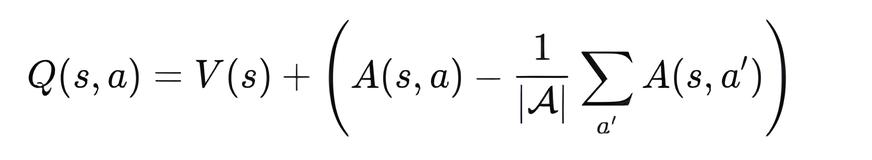
This ensures that the model learns to distinguish between the inherent value of a state (V(s)) and the relative benefit of taking each possible action (A(s, a)), improving stability and performance in value-based reinforcement learning tasks like trading.

# Training loop parameters
env = TradingEnv(xau_data)

# Use positional arguments instead of keyword arguments
model = DuelingDQN(150, 3)  # input_dim=150 (flattened state), action_dim=3
target_model = DuelingDQN(150, 3)  # Same dimensions
target_model.load_state_dict(model.state_dict())

Output:

<All keys matched successfully>

Here we initialize the training environment and models for a Dueling Deep Q-Network (Dueling DQN) agent. The TradingEnv environment is created using the prepared xau_data, which provides market features for reinforcement learning. Two instances of the DuelingDQN model are created: model (the online network) and target_model (the target network), both with a flattened input dimension of 150 and an action space of 3 (buy, sell, hold). The target_model is initialized by copying the weights of model, which is a standard practice in DQN training to stabilize learning by using a slowly updated target network during temporal difference updates.

class ReplayBuffer:
    def __init__(self, capacity=10000):
        self.buffer = deque(maxlen=capacity)

    def push(self, state, action, reward, next_state, done):
        self.buffer.append((state, action, reward, next_state, done))

    def sample(self, batch_size):
        batch = random.sample(self.buffer, batch_size)
        state, action, reward, next_state, done = map(np.array, zip(*batch))
        return (
            torch.tensor(state, dtype=torch.float32),          # Shape: [batch, state_dim]
            torch.tensor(action, dtype=torch.int64),           # Should be integer (for indexing)
            torch.tensor(reward, dtype=torch.float32),         
            torch.tensor(next_state, dtype=torch.float32),
            torch.tensor(done, dtype=torch.float32)
        )

    def __len__(self):
        return len(self.buffer)

The ReplayBuffer class implements a memory buffer used in reinforcement learning to store and sample experiences for training. It uses a deque with a fixed maximum capacity (default: 10,000) to efficiently manage the storage of tuples containing (state, action, reward, next_state, done). The push() method adds new experiences to the buffer, automatically discarding the oldest when the capacity is exceeded.

The sample() method randomly selects a batch of experiences and converts them into PyTorch tensors suitable for model training, ensuring appropriate data types for each element (e.g., int64 for actions and float32 for states and rewards). This buffer supports stable and uncorrelated learning by allowing the agent to learn from a diverse set of past interactions rather than only from consecutive steps.

env = TradingEnv(xau_data)
obs_shape = env.observation_space.shape
n_actions = env.action_space.n

# Calculate flattened dimension
flattened_dim = np.prod(obs_shape)  # 30*5 = 150

model = DuelingDQN(flattened_dim, n_actions)
target_model = DuelingDQN(flattened_dim, n_actions)
target_model.load_state_dict(model.state_dict())

optimizer = optim.Adam(model.parameters(), lr=0.0005)
buffer = ReplayBuffer()
gamma = 0.99
epsilon = 1.0
batch_size = 64
target_update_interval = 10

all_rewards = []
all_actions = []  # We'll collect actions for the entire dataset

# Training loop
for episode in range(200):
    state = env.reset()
    total_reward = 0
    done = False
    episode_actions = []  # Store actions for this episode

    while not done:
        if random.random() < epsilon:
            action = env.action_space.sample()
        else:
            with torch.no_grad():
                # Flatten state and pass to model
                state_tensor = torch.tensor(state, dtype=torch.float32).flatten().unsqueeze(0)
                q_values = model(state_tensor)
                action = q_values.argmax().item()
        
        next_state, reward, done, _ = env.step(action)
        buffer.push(state, action, reward, next_state, done)
        state = next_state
        total_reward += reward
        episode_actions.append(action)  # Record action

        if len(buffer) >= batch_size:
            s, a, r, s2, d = buffer.sample(batch_size)

            q_val = model(s).gather(1, a.unsqueeze(1)).squeeze()
            next_q_val = target_model(s2).max(1)[0]
            target = r + (1 - d) * gamma * next_q_val

            loss = nn.MSELoss()(q_val, target)
            optimizer.zero_grad()
            loss.backward()
            optimizer.step()

    epsilon = max(0.01, epsilon * 0.995)
    if episode % target_update_interval == 0:
        target_model.load_state_dict(model.state_dict())
        print(f"Episode {episode}, Reward: {total_reward}")

    # After episode completes
    all_rewards.append(total_reward)
    all_actions.extend(episode_actions)  # Add episode actions to master list

Output:

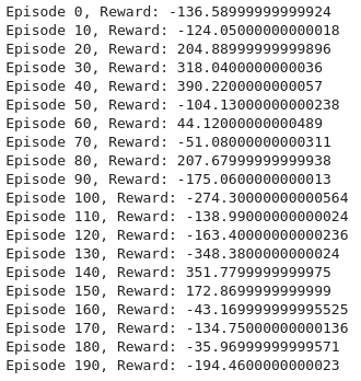
This training loop sets up a reinforcement learning environment for trading using a Dueling Deep Q-Network (Dueling DQN). First, the environment is initialized with historical XAUUSD data, and key parameters are derived from the observation and action spaces. A Dueling DQN model and a target model are created, both with a flattened input shape of 150 (representing 30 time steps × 5 features). An optimizer (Adam) and replay buffer are set up, along with hyperparameters like the discount factor (gamma), exploration rate (epsilon), batch size, and frequency of target network updates.

During each episode, the environment is reset and the agent interacts step-by-step with it by selecting actions using an epsilon-greedy policy. If a random number is less than epsilon, a random action is chosen; otherwise, the model selects the action with the highest predicted Q-value. After executing the action, the agent receives feedback from the environment, which is stored in the replay buffer. Once the buffer has enough data, a batch of experiences is sampled to train the model. The Q-values and targets are computed, and the mean squared error loss is backpropagated to update the model parameters.

To stabilize training, the target model is periodically updated to match the current model's weights. Epsilon is decayed gradually to reduce exploration over time, allowing the agent to exploit learned knowledge more confidently. Throughout training, total rewards and actions per episode are logged for performance evaluation. This loop helps the agent learn an optimal trading strategy by balancing exploration and exploitation over 200 episodes.

import matplotlib.pyplot as plt

# Plotting performance metrics like cumulative reward
plt.plot([r for r in range(len(buffer.buffer))], label="Reward Trend")
plt.title("Training Rewards")
plt.show()

Output:

Here we use matplotlib to visualize the training performance by plotting the reward trend over time based on the entries in the replay buffer. It helps track how the agent's cumulative rewards evolve during training.

import matplotlib.pyplot as plt

plt.figure(figsize=(12, 6))
plt.plot(all_rewards)
plt.xlabel("Episode")
plt.ylabel("Total Reward")
plt.title("Training Performance")
plt.grid(True)
plt.show()

Output:

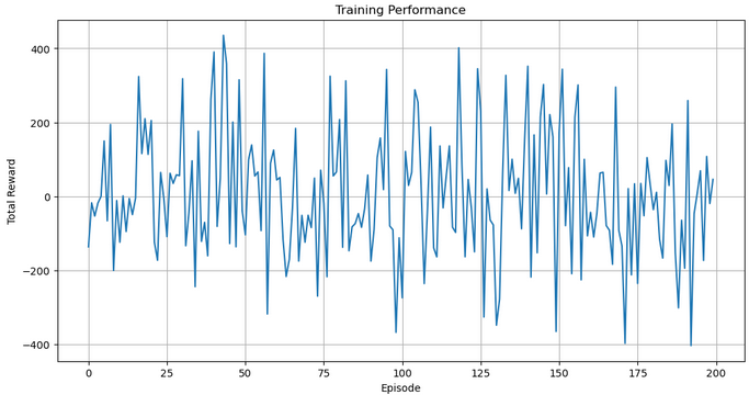
We then visualize the agent’s performance across episodes by plotting all_rewards, which stores the total reward collected in each episode. The plot provides insight into the learning progress and stability of the trading agent over time, with a grid and clear labels for readability.

# Run a clean evaluation with the trained model (no exploration)
eval_env = TradingEnv(xau_data)
state = eval_env.reset()
eval_actions = []  # Store actions for this single episode

with torch.no_grad():
    while True:
        # Flatten state and predict
        state_tensor = torch.tensor(state, dtype=torch.float32).flatten().unsqueeze(0)
        q_values = model(state_tensor)
        action = q_values.argmax().item()
        
        next_state, _, done, _ = eval_env.step(action)
        eval_actions.append(action)
        state = next_state
        
        if done:
            break

# Now plot using eval_actions
close_prices = xau_data['<CLOSE>'].values
window_size = eval_env.observation_space.shape[0]

# Create action array with same length as price data
action_array = np.full(len(close_prices), np.nan)
action_array[window_size:window_size + len(eval_actions)] = eval_actions

# Create plot
plt.figure(figsize=(14, 8))
plt.plot(close_prices, label='XAUUSD Price', alpha=0.7)

# Plot buy signals (action=1)
buy_mask = (action_array == 1)
buy_indices = np.where(buy_mask)[0]
plt.scatter(buy_indices, close_prices[buy_mask], 
            color='green', label='Buy', marker='^', s=100)

# Plot sell signals (action=2)
sell_mask = (action_array == 2)
sell_indices = np.where(sell_mask)[0]
plt.scatter(sell_indices, close_prices[sell_mask], 
            color='red', label='Sell', marker='v', s=100)

plt.legend()
plt.title("Trading Actions on XAUUSD (Trained Policy)")
plt.xlabel("Time Step")
plt.ylabel("Price")
plt.grid(True)
plt.show()

Output:

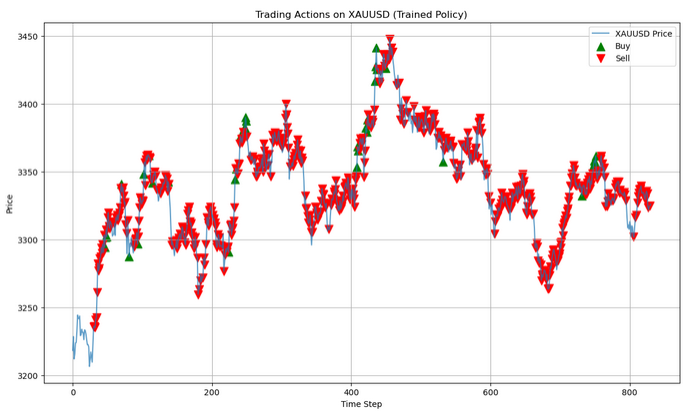
In this evaluation phase, the trained model is used to make predictions in a clean, exploration-free environment (eval_env). The agent observes the market state, selects the best action based on its learned Q-values (greedily choosing the highest), and records each action taken. This loop continues until the episode ends, allowing the agent to demonstrate its learned policy without randomness.

dummy_input = torch.randn(1, *obs_shape)
torch.onnx.export(model, dummy_input, "dueling_dqn_xauusd.onnx",
                  input_names=["input"], output_names=["output"],
                  dynamic_axes={"input": {0: "batch_size"}, "output": {0: "batch_size"}}

Lastly, the trained Dueling DQN model is exported to the ONNX format using a dummy input for compatibility with other platforms. This enables deployment of the trading model outside of PyTorch, such as in real-time systems or MQL5 environments.

Putting it all together on MQL5

//+------------------------------------------------------------------+
//|                                  ONNX_DQN_Trading_Script.mq5     |
//|                        Copyright 2023, MetaQuotes Ltd.           |
//|                                             https://www.mql5.com |
//+------------------------------------------------------------------+
#property copyright "Copyright 2023, MetaQuotes Ltd."
#property link      "https://www.mql5.com"
#property version   "1.00"
#property script_show_inputs

//--- input parameters
input string   ModelPath = "dueling_dqn_xauusd.onnx";  // File in MQL5\Files\
input int      WindowSize = 30;                        // Observation window size
input int      FeatureCount = 5;                       // Number of features

//--- ONNX model handle
long onnxHandle;

//--- Normalization parameters (REPLACE WITH YOUR ACTUAL VALUES)
const double   RSI_MEAN = 55.0,       RSI_STD = 15.0;
const double   MACD_MEAN = 0.05,      MACD_STD = 0.5;
const double   SMA20_MEAN = 1800.0,   SMA20_STD = 100.0;
const double   SMA50_MEAN = 1800.0,   SMA50_STD = 100.0;
const double   RETURN_MEAN = 0.0002,  RETURN_STD = 0.01;

//+------------------------------------------------------------------+
//| Script program start function                                    |
//+------------------------------------------------------------------+
void OnStart()
{
   //--- Load ONNX model
   onnxHandle = OnnxCreate(ModelPath, ONNX_DEFAULT);
   if(onnxHandle == INVALID_HANDLE)
   {
      Print("Error loading model: ", GetLastError());
      return;
   }
   
   //--- Prepare input data buffer
   double inputData[];
   ArrayResize(inputData, WindowSize * FeatureCount);
   
   //--- Collect and prepare data
   if(!PrepareInputData(inputData))
   {
      Print("Data preparation failed");
      OnnxRelease(onnxHandle);
      return;
   }
   
   //--- Set input shape (no need to set shape for dynamic axes)
   //--- Run inference
   double outputData[3];
   if(!RunInference(inputData, outputData))
   {
      Print("Inference failed");
      OnnxRelease(onnxHandle);
      return;
   }
   
   //--- Interpret results
   InterpretResults(outputData);
   OnnxRelease(onnxHandle);
}
//+------------------------------------------------------------------+
//| Prepare input data for the model                                 |
//+------------------------------------------------------------------+
bool PrepareInputData(double &inputData[])
{
   //--- Get closing prices
   double closes[];
   int closeCount = WindowSize + 1;
   if(CopyClose(_Symbol, _Period, 0, closeCount, closes) != closeCount)
   {
      Print("Not enough historical data. Requested: ", closeCount, ", Received: ", ArraySize(closes));
      return false;
   }
   
   //--- Calculate returns (percentage changes)
   double returns[];
   ArrayResize(returns, WindowSize);
   for(int i = 0; i < WindowSize; i++)
      returns[i] = (closes[i] - closes[i+1]) / closes[i+1];
   
   //--- Calculate technical indicators
   double rsi[], macd[], sma20[], sma50[];
   if(!CalculateIndicators(rsi, macd, sma20, sma50))
      return false;
   
   //--- Verify indicator array sizes
   if(ArraySize(rsi) < WindowSize || ArraySize(macd) < WindowSize || 
      ArraySize(sma20) < WindowSize || ArraySize(sma50) < WindowSize)
   {
      Print("Indicator data mismatch");
      return false;
   }
   
   //--- Normalize features and fill input data
   int dataIndex = 0;
   for(int i = WindowSize - 1; i >= 0; i--)
   {
      inputData[dataIndex++] = (rsi[i] - RSI_MEAN) / RSI_STD;
      inputData[dataIndex++] = (macd[i] - MACD_MEAN) / MACD_STD;
      inputData[dataIndex++] = (sma20[i] - SMA20_MEAN) / SMA20_STD;
      inputData[dataIndex++] = (sma50[i] - SMA50_MEAN) / SMA50_STD;
      inputData[dataIndex++] = (returns[i] - RETURN_MEAN) / RETURN_STD;
   }
   
   return true;
}
//+------------------------------------------------------------------+
//| Calculate technical indicators                                   |
//+------------------------------------------------------------------+
bool CalculateIndicators(double &rsi[], double &macd[], double &sma20[], double &sma50[])
{
   //--- RSI (14 period)
   int rsiHandle = iRSI(_Symbol, _Period, 14, PRICE_CLOSE);
   if(rsiHandle == INVALID_HANDLE) return false;
   if(CopyBuffer(rsiHandle, 0, 0, WindowSize, rsi) != WindowSize) return false;
   IndicatorRelease(rsiHandle);
   
   //--- MACD (12,26,9)
   int macdHandle = iMACD(_Symbol, _Period, 12, 26, 9, PRICE_CLOSE);
   if(macdHandle == INVALID_HANDLE) return false;
   double macdSignal[];
   if(CopyBuffer(macdHandle, 0, 0, WindowSize, macd) != WindowSize) return false;
   if(CopyBuffer(macdHandle, 1, 0, WindowSize, macdSignal) != WindowSize) return false;
   
   // Calculate MACD difference (histogram)
   for(int i = 0; i < WindowSize; i++)
      macd[i] = macd[i] - macdSignal[i];
   
   IndicatorRelease(macdHandle);
   
   //--- SMA20
   int sma20Handle = iMA(_Symbol, _Period, 20, 0, MODE_SMA, PRICE_CLOSE);
   if(sma20Handle == INVALID_HANDLE) return false;
   if(CopyBuffer(sma20Handle, 0, 0, WindowSize, sma20) != WindowSize) return false;
   IndicatorRelease(sma20Handle);
   
   //--- SMA50
   int sma50Handle = iMA(_Symbol, _Period, 50, 0, MODE_SMA, PRICE_CLOSE);
   if(sma50Handle == INVALID_HANDLE) return false;
   if(CopyBuffer(sma50Handle, 0, 0, WindowSize, sma50) != WindowSize) return false;
   IndicatorRelease(sma50Handle);
   
   return true;
}
//+------------------------------------------------------------------+
//| Run model inference                                              |
//+------------------------------------------------------------------+
bool RunInference(const double &inputData[], double &outputData[])
{
   //--- Run model directly without setting shape (for dynamic axes)
   if(!OnnxRun(onnxHandle, ONNX_DEBUG_LOGS, inputData, outputData))
   {
      Print("Model inference failed: ", GetLastError());
      return false;
   }
   return true;
}
//+------------------------------------------------------------------+
//| Interpret model results                                          |
//+------------------------------------------------------------------+
void InterpretResults(const double &outputData[])
{
   //--- Find best action
   int bestAction = ArrayMaximum(outputData);
   string actionText = "";
   
   switch(bestAction)
   {
      case 0: actionText = "HOLD"; break;
      case 1: actionText = "BUY"; break;
      case 2: actionText = "SELL"; break;
   }
   
   //--- Print results
   Print("Model Output: [HOLD: ", outputData[0], ", BUY: ", outputData[1], ", SELL: ", outputData[2], "]");
   Print("Recommended Action: ", actionText);
}

This MQL5 script, ONNX_DQN_Trading_Script.mq5, is designed to run a trained Dueling DQN model exported in ONNX format to generate trading signals within MetaTrader 5. It starts by loading the ONNX model from the Files directory and prepares the input data based on a fixed observation window. It collects recent price data and calculates several technical indicators RSI, MACD histogram, SMA20, SMA50, and returns them before normalizing them based on predefined mean and standard deviation values. These processed features are reshaped into a 1D array to match the model's expected input format.

Once the input vector is ready, the script performs inference using OnnxRun, returning three output values that represent the predicted Q-values for the actions: HOLD, BUY, and SELL. The action with the highest value is interpreted as the model's recommendation, which is then printed on the terminal. The inference step is wrapped in error checking to ensure robustness, and handles are released once operations are complete to free system resources.

Conclusion

In summary, we developed an adaptive learning and flexible trading model using a Dueling DQN architecture trained on historical XAUUSD data. The model processes a rolling window of technical features including RSI, MACD histogram, SMA20, SMA50, and return percentages normalized based on statistical parameters. Training progress was visualized using cumulative rewards to ensure learning stability. Once trained, the model was exported to ONNX format for integration into MetaTrader 5, where a dedicated MQL5 script loads the model, prepares input data dynamically, runs inference, and interprets the model's recommended action (HOLD, BUY, or SELL) based on the highest output probability.

In conclusion, this end-to-end pipeline offers traders a powerful and automated decision-support system, blending deep reinforcement learning with real-time market data. The system's flexibility allows easy adaptation to new symbols or indicator configurations by adjusting the input features and retraining. By embedding ONNX inference directly into MQL5, traders can deploy intelligent models natively within their platforms, enhancing both strategy execution and market responsiveness without needing external software dependencies.

File Name	Description
Ada_flex.mq5	File containing the MQL5 script that acts as a bridge between a reinforcement learning model trained in Python
Ada_L.ipynb	File containing the notebook to train the model, and save it
XAUUSD_H1.csv	File containing XAUUSD historical price data