
Neural Networks in Trading: Enhancing Transformer Efficiency by Reducing Sharpness (Final Part)

Introduction
In the previous article we got acquainted with the theoretical aspects of the SAMformer (Sharpness-Aware Multivariate Transformer) framework. It is an innovative model designed to address the inherent limitations of traditional Transformers in long-term forecasting tasks for multivariate time series data. Some of the core issues with vanilla Transformers include high training complexity, poor generalization on small datasets, and a tendency to fall into suboptimal local minima. These limitations hinder the applicability of Transformer-based models in scenarios with limited input data and high demands for predictive accuracy.
The key idea behind SAMformer lies in its use of shallow architecture, which reduces computational complexity and helps prevent overfitting. One of its central components is the Sharpness-Aware Minimization (SAM) optimization mechanism, which enhances the model's robustness to slight parameter variations, thereby improving its generalization capability and the quality of the final predictions.
Thanks to these features, SAMformer delivers outstanding forecast performance on both synthetic and real-world time series datasets. The model achieves high accuracy while significantly reducing the number of parameters, making it more efficient and suitable for deployment in resource-constrained environments. These advantages open the door to SAMformer's broad application across domains such as finance, healthcare, supply chain management, and energy—where long-term forecasting plays a crucial role.
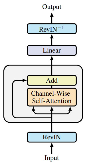
The original visualization of the framework is provided below.
We have already begun implementing the proposed approaches. In the previous article, we introduced new kernels on the OpenCL side. We also discussed enhancements to the fully connected layer. Today, we will continue this work.
1. Convolutional Layer with SAM Optimization
We continue the work we started. As the next step, we are extending the convolutional layer with SAM optimization capabilities. As you might expect, our new class CNeuronConvSAMOCL is implemented as a subclass of the existing convolutional layer CNeuronConvOCL. The structure of the new object is presented below.
class CNeuronConvSAMOCL    :  public CNeuronConvOCL
  {
protected:
   float             fRho;
   //---
   CBufferFloat      cWeightsSAM;
   CBufferFloat      cWeightsSAMConv;
   //---
   virtual bool      calcEpsilonWeights(CNeuronBaseOCL *NeuronOCL);
   virtual bool      feedForwardSAM(CNeuronBaseOCL *NeuronOCL);
   virtual bool      updateInputWeights(CNeuronBaseOCL *NeuronOCL);

public:
                     CNeuronConvSAMOCL(void) {  activation = GELU;   }
                    ~CNeuronConvSAMOCL(void) {};
//---
   virtual bool      Init(uint numOutputs, uint myIndex, COpenCLMy *open_cl,
                          uint window, uint step, uint window_out,
                          uint units_count, uint variables,
                          ENUM_OPTIMIZATION optimization_type, uint batch) override;
   virtual bool      Init(uint numOutputs, uint myIndex, COpenCLMy *open_cl,
                          uint window, uint step, uint window_out,
                          uint units_count, uint variables, float rho,
                          ENUM_OPTIMIZATION optimization_type, uint batch);
   //---
   virtual int       Type(void)   const         {  return defNeuronConvSAMOCL;                         }
   virtual int       Activation(void)  const    {  return (fRho == 0 ? (int)None : (int)activation);   }
   virtual int       getWeightsSAMIndex(void)   {  return cWeightsSAM.GetIndex();                      }
   //--- methods for working with files
   virtual bool      Save(int const file_handle);
   virtual bool      Load(int const file_handle);
   //---
   virtual CLayerDescription* GetLayerInfo(void);
   virtual void      SetOpenCL(COpenCLMy *obj);
  };
Take note that the presented structure includes two buffers for storing adjusted parameters. One buffer is for outgoing connections, similar to the fully connected layer (cWeightsSAM). And another is for incoming connections (cWeightsSAMConv). Note that the parent class does not explicitly include such duplication of parameter buffers. In fact, the buffer for the outgoing connection weights is defined in the parent fully connected layer.
Here, we faced a design dilemma: whether to inherit from the fully connected layer with SAM functionality or from the existing convolutional layer. In the first case, we wouldn't need to define a new buffer for adjusted outgoing connections, as it would be inherited. However, this would require us to completely re-implement the convolutional layer's methods.
In the second scenario, by inheriting from the convolutional layer, we retain all of its existing functionality. However, this approach lacks the buffer for adjusted outgoing weights, which is necessary for the proper operation of the subsequent fully connected SAM-optimized layer.
We chose the second inheritance option, as it required less effort to implement the functionality needed.
As before, we declare additional internal objects statically, allowing us to keep the constructor and destructor empty. Nevertheless, within the class constructor, we set GELU as the default activation function. All remaining initialization steps for both inherited and newly declared objects are carried out in the Init method. Here, you'll notice the overriding of two methods with the same name but different parameter sets. We'll first examine the version with the most comprehensive parameter list.
bool CNeuronConvSAMOCL::Init(uint numOutputs, uint myIndex, COpenCLMy *open_cl,
                             uint window_in, uint step, uint window_out,
                             uint units_count, uint variables, float rho,
                             ENUM_OPTIMIZATION optimization_type, uint batch)
  {
   if(!CNeuronConvOCL::Init(numOutputs, myIndex, open_cl, window_in, step, window_out,
                                    units_count, variables, optimization_type, batch))
      return false;
In the method parameters, we receive the main constants that allow us to uniquely determine the architecture of the object being created. We immediately pass nearly all of these parameters to the parent class method of the same name, where all necessary control points and initialization algorithms for inherited objects have already been implemented.
After the successful execution of the parent class method, we store the blur region coefficient in an internal variable. This is the only parameter we do not pass to the parent method.
   fRho = fabs(rho);
   if(fRho == 0)
      return true;
We then immediately check the stored value. If the blur coefficient is zero, the SAM optimization algorithm degenerates into the base parameter optimization method. In that case, all required components have already been initialized by the parent class. So, we can return a successful result.
Otherwise, we first initialize the buffer for the adjusted incoming connections with zero values.
   cWeightsSAMConv.BufferFree();
   if(!cWeightsSAMConv.BufferInit(WeightsConv.Total(), 0) ||
      !cWeightsSAMConv.BufferCreate(OpenCL))
      return false;
Next, if necessary, we similarly initialize the buffer for adjusted outgoing parameters.
   cWeightsSAM.BufferFree();
   if(!Weights)
     return true;
   if(!cWeightsSAM.BufferInit(Weights.Total(), 0) ||
      !cWeightsSAM.BufferCreate(OpenCL))
      return false;
//---
   return true;
  }
Note that this last buffer is initialized only if outgoing connection parameters are present. This occurs when the convolutional layer is followed by a fully connected layer.
After successfully initializing all internal components, the method returns the logical result of the operation back to the calling program.
The second initialization method in our class completely overrides the parent class method and has identical parameters. However, as you may have guessed, it omits the blur coefficient parameter, which is critical for SAM optimization. In the method body, we assign a default blur coefficient of 0.7. This coefficient was mentioned in the original paper introducing the SAMformer framework. We then call the previously described class initialization method.
bool CNeuronConvSAMOCL::Init(uint numOutputs, uint myIndex, COpenCLMy *open_cl,

                             uint window_in, uint step, uint window_out,
                             uint units_count, uint variables,
                             ENUM_OPTIMIZATION optimization_type, uint batch)
  {
   return CNeuronConvSAMOCL::Init(numOutputs, myIndex, open_cl, window_in, step, window_out, units_count,
                                                                variables, 0.7f, optimization_type, batch);
  }
This approach allows us to easily swap a regular convolutional layer with its SAM-optimized counterpart in nearly any of the previously discussed architectural configurations, simply by changing the object type.
As with the fully connected layer, all forward-pass and gradient distribution functionality is inherited from the parent class. However, we introduce two wrapper methods for calling OpenCL program kernels: calcEpsilonWeights and feedForwardSAM. The first method calls the kernel responsible for computing the adjusted parameters. The second one mirrors the parent forward-pass method but uses the adjusted parameter buffer instead. We will not go into the detailed logic of these methods here. They follow the same kernel-queuing algorithms discussed earlier. You can explore their full implementations in the attached source code.
The parameter optimization method of this class closely resembles its counterpart in the fully connected SAM-optimized layer. However, in this case, we don't check the type of the preceding layer. Unlike fully connected layers, a convolutional layer contains its own internal parameter matrix applied to input data. Thus, it uses its own adjusted parameter buffer. All it needs from the previous layer is the input data buffer, which all of our objects provide.
Nonetheless, we check the blur coefficient value. When it is zero, SAM optimization is effectively bypassed. In this case, we simply use the parent class method.
bool CNeuronConvSAMOCL::updateInputWeights(CNeuronBaseOCL *NeuronOCL)
  {
   if(fRho <= 0)
      return CNeuronConvOCL::updateInputWeights(NeuronOCL);
If SAM optimization is enabled, we first combine the error gradient with the feed-forward pass results to produce the current object's target tensor:
   if(!SumAndNormilize(Gradient, Output, Gradient, iWindowOut, false, 0, 0, 0, 1))
      return false;
Next, we update the model parameters using the blur coefficient. This involves calling the wrapper that enqueues the appropriate kernel. Note that both convolutional and fully connected layers use methods with identical names. But they are queued to different kernels specific to their internal architectures.
   if(!calcEpsilonWeights(NeuronOCL))
      return false;
The same applies to the feed-forward methods using adjusted parameters.
   if(!feedForwardSAM(NeuronOCL))
      return false;
After a successful second feed-forward pass, we calculate the deviation from the target values.
   float error = 1;
   if(!calcOutputGradients(Gradient, error))
      return false;
We then call the parent class’s method to update the model’s parameters.
//---
   return CNeuronConvOCL::updateInputWeights(NeuronOCL);
  }
Finally, the logical result is returned to the calling program, completing the method.
A few words need to be said about saving the parameters of the trained model. When saving the trained model, we follow the same approach discussed in the context of the fully connected SAM layer. We do not save the buffers containing adjusted parameters. Instead, we only add the blur coefficient to the data saved by the parent class.
bool CNeuronConvSAMOCL::Save(const int file_handle)
  {
   if(!CNeuronConvOCL::Save(file_handle))
      return false;
   if(FileWriteFloat(file_handle, fRho) < INT_VALUE)
      return false;
//---
   return true;
  }
When loading a pre-trained model, we need to prepare the necessary buffers. It's important to note that the criteria for creating buffers for adjusted incoming and outgoing parameters are different.
First, we load the data saved by the parent class.
bool CNeuronConvSAMOCL::Load(const int file_handle)
  {
   if(!CNeuronConvOCL::Load(file_handle))
      return false;
Next, we check whether the file contains more data, then read the blur coefficient.
   if(FileIsEnding(file_handle))
      return false;
   fRho = FileReadFloat(file_handle);
A positive blur coefficient is the key condition for initializing the adjusted parameter buffers. So, we check the value of the loaded parameter. If this condition is not met, we clear any unused buffers in the OpenCL context and in the main memory. After that we complete the method with a positive result.
   cWeightsSAMConv.BufferFree();
   cWeightsSAM.BufferFree();
   cWeightsSAMConv.Clear();
   cWeightsSAM.Clear();
   if(fRho <= 0)
      return true;
This is one of those cases where the control point is non-critical to program execution. As noted earlier, a zero blur coefficient reduces SAM to a basic optimization method. So, in that case, our object falls back to the functionality of the parent class.
If the condition is satisfied, we proceed to initialize and allocate memory in the OpenCL context for the adjusted incoming parameters.
   if(!cWeightsSAMConv.BufferInit(WeightsConv.Total(), 0) ||
      !cWeightsSAMConv.BufferCreate(OpenCL))
      return false;
To create the buffer for adjusted outgoing parameters, an additional condition must be met: the presence of such connections. Therefore, we check the pointer validity before initialization.
   if(!Weights)
     return true;
Again, lack of a valid pointer is not a critical error. It simply reflects the architecture of the model. Therefore, if there is no current pointer, we terminate the method with a positive result.
In an outgoing connection buffer is found, we initialize and create a similarly sized buffer for the adjusted parameters.
   if(!cWeightsSAM.BufferInit(Weights.Total(), 0) ||
      !cWeightsSAM.BufferCreate(OpenCL))
      return false;
//---
   return true;
  }
Then we return the logical result of the operation to the caller and complete the method execution.
With this, we complete our examination of the convolutional layer methods implementing SAM optimization in CNeuronConvSAMOCL. The full code of this class and all its methods can be found in the attachment.
2. Adding SAM to the Transformer
At this stage, we have created both fully connected and convolutional layer objects that incorporate SAM-based parameter optimization. It is now time to integrate these approaches into the Transformer architecture. This is exactly as proposed by the authors of the SAMformer framework. To objectively evaluate the impact of these techniques on model performance, we decided not to create entirely new classes. Instead, we integrated the SAM-based approaches directly into the structure of an existing class For the base architecture, we chose the Transformer with relative attention R-MAT.
As you know, the CNeuronRMAT class implements a linear sequence of alternating CNeuronRelativeSelfAttention and CResidualConv objects. The first implements the relative attention mechanism with feedback, while the second contains a feedback-based convolutional block. To integrate SAM optimization, it is sufficient to replace all convolutional layers in these objects with their SAM-enabled counterparts. The updated class structure is shown below.
class CNeuronRelativeSelfAttention   :  public CNeuronBaseOCL
  {
protected:
   uint                    iWindow;
   uint                    iWindowKey;
   uint                    iHeads;
   uint                    iUnits;
   int                     iScore;
   //---
   CNeuronConvSAMOCL          cQuery;
   CNeuronConvSAMOCL          cKey;
   CNeuronConvSAMOCL          cValue;
   CNeuronTransposeOCL     cTranspose;
   CNeuronBaseOCL          cDistance;
   CLayer                  cBKey;
   CLayer                  cBValue;
   CLayer                  cGlobalContentBias;
   CLayer                  cGlobalPositionalBias;
   CLayer                  cMHAttentionPooling;
   CLayer                  cScale;
   CBufferFloat            cTemp;
   //---
   virtual bool      AttentionOut(void);
   virtual bool      AttentionGradient(void);

   //---
   virtual bool      feedForward(CNeuronBaseOCL *NeuronOCL) override;
   virtual bool      calcInputGradients(CNeuronBaseOCL *NeuronOCL) override;
   virtual bool      updateInputWeights(CNeuronBaseOCL *NeuronOCL) override;

public:
                     CNeuronRelativeSelfAttention(void) : iScore(-1) {};
                    ~CNeuronRelativeSelfAttention(void) {};
   //---
   virtual bool      Init(uint numOutputs, uint myIndex, COpenCLMy *open_cl,
                          uint window, uint window_key,
                          uint units_count, uint heads,
                          ENUM_OPTIMIZATION optimization_type, uint batch);
   //---
   virtual int       Type(void) override   const   {  return defNeuronRelativeSelfAttention; }
   //---
   virtual bool      Save(int const file_handle) override;
   virtual bool      Load(int const file_handle) override;
   //---
   virtual bool      WeightsUpdate(CNeuronBaseOCL *source, float tau) override;
   virtual void      SetOpenCL(COpenCLMy *obj) override;
   //---
   virtual uint      GetWindow(void) const { return iWindow; }
   virtual uint      GetUnits(void) const { return iUnits; }
  };
class CResidualConv  :  public CNeuronBaseOCL
  {
protected:
   int               iWindowOut;
   //---
   CNeuronConvSAMOCL    cConvs[3];
   CNeuronBatchNormOCL cNorm[3];
   CNeuronBaseOCL    cTemp;
   //---
   virtual bool      feedForward(CNeuronBaseOCL *NeuronOCL);
   virtual bool      updateInputWeights(CNeuronBaseOCL *NeuronOCL);
   virtual bool      calcInputGradients(CNeuronBaseOCL *prevLayer);

public:
                     CResidualConv(void) {};
                    ~CResidualConv(void) {};
   //---
   virtual bool      Init(uint numOutputs, uint myIndex, COpenCLMy *open_cl,
                          uint window, uint window_out, uint count,
                          ENUM_OPTIMIZATION optimization_type,
                          uint batch);
   //---
   virtual int       Type(void)   const   {  return defResidualConv;   }
   //--- methods for working with files
   virtual bool      Save(int const file_handle);
   virtual bool      Load(int const file_handle);
   virtual CLayerDescription* GetLayerInfo(void);
   virtual void      SetOpenCL(COpenCLMy *obj);
   virtual void      TrainMode(bool flag);
  };
Note that for the feedback convolutional module, we only modify the object type in the class structure. No changes are required to the class methods. This is possible because of our overloaded convolutional layer initialization methods with SAM initialization. Recall that the CNeuronConvSAMOCL class provides two initialization methods: one with the blur coefficient as a parameter and one without it. The method without the blur coefficient overrides the parent class method previously used to initialize convolutional layers. As a result, when initializing CResidualConv objects, the program calls our overridden initialization method, which automatically assigns a default blur coefficient and triggers full convolutional layer initialization with SAM optimization.
The situation with the relative attention module is slightly more complex. The CNeuronRelativeSelfAttention module has a more complex architecture that includes additional nested trainable bias models. Their architecture is defined in the object initialization method. Therefore, to enable SAM optimization for these internal models, we must modify the initialization method of the relative attention module itself.
The method parameters remain unchanged, and the initial steps of its algorithm are also preserved. The object types for generating the Query, Key, and Value entities have already been updated in the class structure.
bool CNeuronRelativeSelfAttention::Init(uint numOutputs, uint myIndex, COpenCLMy *open_cl,
                               uint window, uint window_key, uint units_count, uint heads,
                                          ENUM_OPTIMIZATION optimization_type, uint batch)
  {
   if(!CNeuronBaseOCL::Init(numOutputs, myIndex, open_cl, window * units_count, optimization_type, batch))
      return false;
//---
   iWindow = window;
   iWindowKey = window_key;
   iUnits = units_count;
   iHeads = heads;
//---
   int idx = 0;
   if(!cQuery.Init(0, idx, OpenCL, iWindow, iWindow, iWindowKey * iHeads, iUnits, 1, optimization, iBatch))
      return false;
   cQuery.SetActivationFunction(GELU);
   idx++;
   if(!cKey.Init(0, idx, OpenCL, iWindow, iWindow, iWindowKey * iHeads, iUnits, 1, optimization, iBatch))
      return false;
   cKey.SetActivationFunction(GELU);
   idx++;
   if(!cValue.Init(0, idx, OpenCL, iWindow, iWindow, iWindowKey * iHeads, iUnits, 1, optimization, iBatch))
      return false;
   cKey.SetActivationFunction(GELU);
   idx++;
   if(!cTranspose.Init(0, idx, OpenCL, iUnits, iWindow, optimization, iBatch))
      return false;
   idx++;
   if(!cDistance.Init(0, idx, OpenCL, iUnits * iUnits, optimization, iBatch))
      return false;
Further, in the BKey and BValue bias generation models, we substitute convolutional object types while maintaining other parameters.
   idx++;
   CNeuronConvSAMOCL *conv = new CNeuronConvSAMOCL();
   if(!conv ||
      !conv.Init(0, idx, OpenCL, iUnits, iUnits, iWindow, iUnits, 1, optimization, iBatch) ||
      !cBKey.Add(conv))
      return false;
   idx++;
   conv.SetActivationFunction(TANH);
   conv = new CNeuronConvSAMOCL();
   if(!conv ||
      !conv.Init(0, idx, OpenCL, iWindow, iWindow, iWindowKey * iHeads, iUnits, 1, optimization, iBatch) ||
      !cBKey.Add(conv))
      return false;
   idx++;
   conv = new CNeuronConvSAMOCL();
   if(!conv ||
      !conv.Init(0, idx, OpenCL, iUnits, iUnits, iWindow, iUnits, 1, optimization, iBatch) ||
      !cBValue.Add(conv))
      return false;
   idx++;
   conv.SetActivationFunction(TANH);
   conv = new CNeuronConvSAMOCL();
   if(!conv ||
      !conv.Init(0, idx, OpenCL, iWindow, iWindow, iWindowKey * iHeads, iUnits, 1, optimization, iBatch) ||
      !cBValue.Add(conv))
      return false;
In the models for generating global context and position biases, we use fully connected layers with SAM optimization.
   idx++;
   CNeuronBaseOCL *neuron = new CNeuronBaseSAMOCL();
   if(!neuron ||
      !neuron.Init(iWindowKey * iHeads * iUnits, idx, OpenCL, 1, optimization, iBatch) ||
      !cGlobalContentBias.Add(neuron))
      return false;
   idx++;
   CBufferFloat *buffer = neuron.getOutput();
   buffer.BufferInit(1, 1);
   if(!buffer.BufferWrite())
      return false;
   neuron = new CNeuronBaseSAMOCL();
   if(!neuron ||
      !neuron.Init(0, idx, OpenCL, iWindowKey * iHeads * iUnits, optimization, iBatch) ||
      !cGlobalContentBias.Add(neuron))
      return false;
   idx++;
   neuron = new CNeuronBaseSAMOCL();
   if(!neuron ||
      !neuron.Init(iWindowKey * iHeads * iUnits, idx, OpenCL, 1, optimization, iBatch) ||
      !cGlobalPositionalBias.Add(neuron))
      return false;
   idx++;
   buffer = neuron.getOutput();
   buffer.BufferInit(1, 1);
   if(!buffer.BufferWrite())
      return false;
   neuron = new CNeuronBaseSAMOCL();
   if(!neuron ||
      !neuron.Init(0, idx, OpenCL, iWindowKey * iHeads * iUnits, optimization, iBatch) ||
      !cGlobalPositionalBias.Add(neuron))
      return false;
For pooling operation MLP, we again use convolutional layers using SAM optimization approaches.
   idx++;
   neuron = new CNeuronBaseOCL();
   if(!neuron ||
      !neuron.Init(0, idx, OpenCL, iWindowKey * iHeads * iUnits, optimization, iBatch) ||
      !cMHAttentionPooling.Add(neuron)
     )
      return false;
   idx++;
   conv = new CNeuronConvSAMOCL();
   if(!conv ||
      !conv.Init(0, idx, OpenCL, iWindowKey * iHeads, iWindowKey * iHeads, iWindow, iUnits, 1, optimization, iBatch) ||
      !cMHAttentionPooling.Add(conv)
     )
      return false;
   idx++;
   conv.SetActivationFunction(TANH);
   conv = new CNeuronConvSAMOCL();
   if(!conv ||
      !conv.Init(0, idx, OpenCL, iWindow, iWindow, iHeads, iUnits, 1, optimization, iBatch) ||
      !cMHAttentionPooling.Add(conv)
     )
      return false;
   idx++;
   conv.SetActivationFunction(None);
   CNeuronSoftMaxOCL *softmax = new CNeuronSoftMaxOCL();
   if(!softmax ||
      !softmax.Init(0, idx, OpenCL, iHeads * iUnits, optimization, iBatch) ||
      !cMHAttentionPooling.Add(softmax)
     )
      return false;
   softmax.SetHeads(iUnits);
Note that for the first layer, we still use the base fully connected layer. Because it is used solely to store the output of the multi-head attention block.
A similar situation occurs in the scaling block. The first layer remains a base fully connected layer, as it stores the result of multiplying attention weights by the outputs of the multi-head attention block. This is then followed by convolutional layers with SAM optimization.
   idx++;
   neuron = new CNeuronBaseOCL();
   if(!neuron ||
      !neuron.Init(0, idx, OpenCL, iWindowKey * iUnits, optimization, iBatch) ||
      !cScale.Add(neuron)
     )
      return false;
   idx++;
   conv = new CNeuronConvSAMOCL();
   if(!conv ||
      !conv.Init(0, idx, OpenCL, iWindowKey, iWindowKey, 2 * iWindow, iUnits, 1, optimization, iBatch) ||
      !cScale.Add(conv)
     )
      return false;
   conv.SetActivationFunction(LReLU);
   idx++;
   conv = new CNeuronConvSAMOCL();
   if(!conv ||
      !conv.Init(0, idx, OpenCL,
2  * iWindow, 2 * iWindow, iWindow, iUnits, 1, optimization, iBatch) ||
      !cScale.Add(conv)
     )
      return false;
   conv.SetActivationFunction(None);
//---
   if(!SetGradient(conv.getGradient(), true))
      return false;
//---
   SetOpenCL(OpenCL);
//---
   return true;
  }
With that, we conclude the integration of SAM optimization approaches into the Transformer with relative attention. The full code for the updated objects is provided in the attachment.
3. Model Architecture
We have created new objects and updated certain existing ones. The next step is to adjust the overall model architecture. Unlike in some recent articles, today's architectural changes are more extensive. We begin with the architecture of the environment Encoder, implemented in the CreateEncoderDescriptions method. As before, this method receives a pointer to a dynamic array where the sequence of model layers will be recorded.
bool CreateEncoderDescriptions(CArrayObj *&encoder)
  {
//---
   CLayerDescription *descr;
//---
   if(!encoder)
     {
      encoder = new CArrayObj();
      if(!encoder)
         return false;
     }
In the method body, we check the relevance of the received pointer and, if necessary, create a new instance of the dynamic array.
We leave the first 2 layers unchanged. These are the source data and batch normalization layers. The size of these layers is identical and must be sufficient to record the original data tensor.
//--- Encoder
   encoder.Clear();
//--- Input layer
   if(!(descr = new CLayerDescription()))
      return false;
   descr.type = defNeuronBaseOCL;
   int prev_count = descr.count = (HistoryBars * BarDescr);
   descr.activation = None;
   descr.optimization = ADAM;
   if(!encoder.Add(descr))
     {
      delete descr;
      return false;
     }
//--- layer 1
   if(!(descr = new CLayerDescription()))
      return false;
   descr.type = defNeuronBatchNormOCL;
   descr.count = prev_count;
   descr.batch = 1e4;
   descr.activation = None;
   descr.optimization = ADAM;
   if(!encoder.Add(descr))
     {
      delete descr;
      return false;
     }
Next, the authors of the SAMformer framework propose using attention by channels. Therefore, we use a data transposition layer that helps us represent the original data as a sequence of attention channels.
//--- layer 2
   if(!(descr = new CLayerDescription()))
      return false;
   descr.type = defNeuronTransposeOCL;
   descr.count = HistoryBars;
   descr.window= BarDescr;
   descr.activation = None;
   descr.optimization = ADAM;
   if(!encoder.Add(descr))
     {
      delete descr;
      return false;
     }
Then we use the relative attention block, into which we have already added SAM optimization approaches.
//--- layer 3
   if(!(descr = new CLayerDescription()))
      return false;
   descr.type = defNeuronRMAT;
   descr.window=HistoryBars;
   descr.count=BarDescr;
   descr.window_out = EmbeddingSize/2;                // Key Dimension
   descr.layers = 1;                                  // Layers
   descr.step = 2;                                    // Heads
   descr.batch = 1e4;
   descr.activation = None;
   descr.optimization = ADAM;
   if(!encoder.Add(descr))
     {
      delete descr;
      return false;
     }
Two important points should be noted here. First, we use channel attention. Therefore, the analysis window equals the depth of the analyzed history, and the number of elements matches the number of independent channels. Second, as proposed by the authors of the SAMformer framework, we use only one attention layer. However, unlike the original implementation, we employ two attention heads. We have also retained the FeedForward block. Although, the framework authors used only one attention head and removed the FeedForward component.
Next, we must reduce the dimensionality of the output tensor to the desired size. This will be done in two stages. First, we apply a convolutional layer with SAM optimization to reduce the dimensionality of the individual channels.
//--- layer 4
   if(!(descr = new CLayerDescription()))
      return false;
   descr.type = defNeuronConvSAMOCL;
   descr.count = BarDescr;
   descr.window = HistoryBars;
   descr.step = HistoryBars;
   descr.window_out = LatentCount/BarDescr;
   descr.probability = 0.7f;
   descr.activation = GELU;
   descr.optimization = ADAM;
   if(!encoder.Add(descr))
     {
      delete descr;
      return false;
     }
Then we use a fully connected layer with SAM optimization to obtain a general embedding of the current environmental state of a given size.
//--- layer 5
   if(!(descr = new CLayerDescription()))
      return false;
   descr.type = defNeuronBaseSAMOCL;
   descr.count = LatentCount;
   descr.probability = 0.7f;
   descr.activation = None;
   descr.optimization = ADAM;
   if(!encoder.Add(descr))
     {
      delete descr;
      return false;
     }
//---
   return true;
  }
In both cases we use descr.probability to specify the blur area coefficient.
The method concludes by returning the logical result of the operation to the caller. The model architecture itself is returned via the dynamic array pointer provided as a parameter.
After defining the architecture of the environment Encoder, we proceed to describe the layers of the Actor and Critic layers. The descriptions of both models are generated in the CreateDescriptions method. Since this method builds two separate model descriptions, its parameters include two pointers to dynamic arrays.
bool CreateDescriptions(CArrayObj *&actor, CArrayObj *&critic)
  {
//---
   CLayerDescription *descr;
//---
   if(!actor)
     {
      actor = new CArrayObj();
      if(!actor)
         return false;
     }
   if(!critic)
     {
      critic = new CArrayObj();
      if(!critic)
         return false;
     }
Inside the method, we verify the validity of the provided pointers and, if necessary, create new dynamic arrays.
We start with the architecture of the Actor. The first layer of this model is implemented as a fully connected layer with SAM optimization. Its size matches the state description vector of the trading account.
//--- Actor
   actor.Clear();
//--- Input layer
   if(!(descr = new CLayerDescription()))
      return false;
   descr.type = defNeuronBaseSAMOCL;
   int prev_count = descr.count = AccountDescr;
   descr.activation = None;
   descr.probability=0.7f;
   descr.optimization = ADAM;
   if(!actor.Add(descr))
     {
      delete descr;
      return false;
     }
It is worth noting that here, we use a SAM-optimized fully connected layer to record the input data. In the environment Encoder, a base fully connected layer was used in a similar position. This difference is due to the presence of a subsequent fully connected layer with SAM optimization, which requires the preceding layer to provide a buffer of adjusted parameters for correct operation.
//--- layer 1
   if(!(descr = new CLayerDescription()))
      return false;
   descr.type = defNeuronBaseSAMOCL;
   prev_count = descr.count = EmbeddingSize;
   descr.activation = SIGMOID;
   descr.optimization = ADAM;
   descr.probability=0.7f;
   if(!actor.Add(descr))
     {
      delete descr;
      return false;
     }
As in the environment encoder, we use descr.probability to set the blur region coefficient. For all models, we apply a unified coefficient of 0.7.
Two consecutive SAM-optimized fully connected layers create embeddings of the current trading account state, which are then concatenated with the corresponding environmental state embedding. This concatenation is performed by a dedicated data concatenation layer.
//--- layer 2
   if(!(descr = new CLayerDescription()))
      return false;
   descr.type = defNeuronConcatenate;
   descr.count = LatentCount;
   descr.window = EmbeddingSize;
   descr.step = LatentCount;
   descr.activation = LReLU;
   descr.optimization = ADAM;
   if(!actor.Add(descr))
     {
      delete descr;
      return false;
     }
The result is passed to a decision-making block consisting of three SAM-optimized fully connected layers.
//--- layer 3
   if(!(descr = new CLayerDescription()))
      return false;
   descr.type = defNeuronBaseSAMOCL;
   descr.count = LatentCount;
   descr.activation = SIGMOID;
   descr.optimization = ADAM;
   descr.probability=0.7f;
   if(!actor.Add(descr))
     {
      delete descr;
      return false;
     }
//--- layer 4
   if(!(descr = new CLayerDescription()))
      return false;
   descr.type = defNeuronBaseSAMOCL;
   descr.count = LatentCount;
   descr.activation = SIGMOID;
   descr.optimization = ADAM;
   descr.probability=0.7f;
   if(!actor.Add(descr))
     {
      delete descr;
      return false;
     }
//--- layer 5
   if(!(descr = new CLayerDescription()))
      return false;
   descr.type = defNeuronBaseSAMOCL;
   descr.count = 2 * NActions;
   descr.activation = None;
   descr.optimization = ADAM;
   descr.probability=0.7f;
   if(!actor.Add(descr))
     {
      delete descr;
      return false;
     }
At the output of the final layer, we generate a tensor that is twice the size of the Actor’s target action vector. This design allows us to incorporate stochasticity into the actions. As before, we achieve this using the latent state layer of an autoencoder.
//--- layer 6
   if(!(descr = new CLayerDescription()))
      return false;
   descr.type = defNeuronVAEOCL;
   descr.count = NActions;
   descr.optimization = ADAM;
   if(!actor.Add(descr))
     {
      delete descr;
      return false;
     }
Recall that the latent layer of an autoencoder splits the input tensor into two parts: the first part contains the mean values of the distributions for each element of the output sequence, and the second part contains the variances of the corresponding distributions. Training these means and variances within the decision-making module enables us to constrain the range of generated random values via the latent layer of the autoencoder, thus introducing stochasticity into the Actor's policy.
It is worth adding that the autoencoder's latent layer generates independent values for each element of the output sequence. However, in our case, we expect a coherent set of parameters for executing a trade: position size, take-profit levels, and stop-loss levels. To ensure consistency among these trade parameters, we employ a SAM-optimized convolutional layer that separately analyzes the parameters for long and short trades.
//--- layer 7
   if(!(descr = new CLayerDescription()))
      return false;
   descr.type = defNeuronConvSAMOCL;
   descr.count = NActions / 3;
   descr.window = 3;
   descr.step = 3;
   descr.window_out = 3;
   descr.activation = SIGMOID;
   descr.optimization = ADAM;
   descr.probability=0.7f;
   if(!actor.Add(descr))
     {
      delete descr;
      return false;
     }
To limit the output domain of this layer, we use a sigmoid activation function.
And the final touch of our Actor model is a frequency-boosted feed-forward prediction layer (CNeuronFreDFOCL), which allows the results of the model to be matched with the target values in the frequency domain.
//--- layer 8
   if(!(descr = new CLayerDescription()))
      return false;
   descr.type = defNeuronFreDFOCL;
   descr.window = NActions;
   descr.count =  1;
   descr.step = int(false);
   descr.probability = 0.7f;
   descr.activation = None;
   descr.optimization = ADAM;
   if(!actor.Add(descr))
     {
      delete descr;
      return false;
     }
The Critic model has a similar architecture. However, instead of describing the state of the account passed to the Actor, we feed the model with the parameters of the trading operation generated by the Actor. We also use 2 fully connected layers with SAM optimization to obtain trading operation embedding.
//--- Critic
   critic.Clear();
//--- Input layer
   if(!(descr = new CLayerDescription()))
      return false;
   descr.type = defNeuronBaseSAMOCL;
   prev_count = descr.count = NActions;
   descr.activation = None;
   descr.optimization = ADAM;
   descr.probability=0.7f;
   if(!critic.Add(descr))
     {
      delete descr;
      return false;
     }
//--- layer 1
   if(!(descr = new CLayerDescription()))
      return false;
   descr.type = defNeuronBaseSAMOCL;
   prev_count = descr.count = EmbeddingSize;
   descr.activation = SIGMOID;
   descr.optimization = ADAM;
   descr.probability=0.7f;
   if(!critic.Add(descr))
     {
      delete descr;
      return false;
     }
The trading operation embedding is combined with the environment state embedding in the data concatenation layer.
//--- layer 2
   if(!(descr = new CLayerDescription()))
      return false;
   descr.type = defNeuronConcatenate;
   descr.count = LatentCount;
   descr.window = EmbeddingSize;
   descr.step = LatentCount;
   descr.activation = LReLU;
   descr.optimization = ADAM;
   if(!critic.Add(descr))
     {
      delete descr;
      return false;
     }
And then we use a decision block of 3 consecutive fully connected layers with SAM optimization. But unlike Actor, in this case the stochastic nature of the results is not used.
//--- layer 3
   if(!(descr = new CLayerDescription()))
      return false;
   descr.type = defNeuronBaseSAMOCL;
   descr.count = LatentCount;
   descr.activation = SIGMOID;
   descr.optimization = ADAM;
   descr.probability=0.7f;
   if(!critic.Add(descr))
     {
      delete descr;
      return false;
     }
//--- layer 4
   if(!(descr = new CLayerDescription()))
      return false;
   descr.type = defNeuronBaseSAMOCL;
   descr.count = LatentCount;
   descr.activation = SIGMOID;
   descr.optimization = ADAM;
   descr.probability=0.7f;
   if(!critic.Add(descr))
     {
      delete descr;
      return false;
     }
//--- layer 5
   if(!(descr = new CLayerDescription()))
      return false;
   descr.type = defNeuronBaseSAMOCL;
   descr.count = LatentCount;
   descr.activation = SIGMOID;
   descr.optimization = ADAM;
   descr.probability=0.7f;
   if(!critic.Add(descr))
     {
      delete descr;
      return false;
     }
//--- layer 6
   if(!(descr = new CLayerDescription()))
      return false;
   descr.type = defNeuronBaseSAMOCL;
   descr.count = NRewards;
   descr.activation = None;
   descr.optimization = ADAM;
   descr.probability=0.7f;
   if(!critic.Add(descr))
     {
      delete descr;
      return false;
     }
On top of the Critic model, we add a forward prediction layer with frequency gain.
//--- layer 7
   if(!(descr = new CLayerDescription()))
      return false;
   descr.type = defNeuronFreDFOCL;
   descr.window = NRewards;
   descr.count =  1;
   descr.step = int(false);
   descr.probability = 0.7f;
   descr.activation = None;
   descr.optimization = ADAM;
   if(!critic.Add(descr))
     {
      delete descr;
      return false;
     }
//---
   return true;
  }
After completing the generation of the model architecture descriptions, the method terminates by returning the logical result of the operations to the caller. The architecture descriptions themselves are returned via the dynamic array pointers received in the method parameters.
This concludes our work on model construction. The complete architecture can be found in the attachments. There you will also find the full source code for the environment interaction and model training programs, which have been carried over from previous work without modification.
4. Testing
We have carried out a substantial amount of work implementing the approaches proposed by the authors of the SAMformer framework. It is now time to evaluate the effectiveness of our implementation on real historical data. As before, model training was conducted on actual historical data for the EURUSD instrument covering the entire year of 2023. Throughout the experiments, we used the H1 timeframe. All indicator parameters were set to their default values.
As mentioned earlier, the programs responsible for environment interaction and model training remained unchanged. This allows us to reuse the training datasets created earlier for the initial training of our models. Moreover, since the R-MAT framework was chosen as the baseline for incorporating SAM optimization, we decided not to update the training set during model training. Naturally, we expect this choice to have a negative impact on model performance. However, it enables a more direct comparison with the baseline model by removing any influence from changes in the training dataset.
Training for all three models was conducted simultaneously. The results of testing the trained Actor policy are presented below. The testing was performed on real historical data for January 2024, with all other training parameters unchanged.
Before examining the results, I would like to mention several points regarding model training. First, SAM optimization inherently smooths the loss landscape. This, in turn, allows us to consider higher learning rates. While in earlier works we primarily used a learning rate of 3.0e-04, in this case we increased it to 1.0e-03.
Second, the use of only a single attention layer reduced the total number of trainable parameters, helping to offset the computational overhead introduced by the additional feed-forward pass required by SAM optimization.
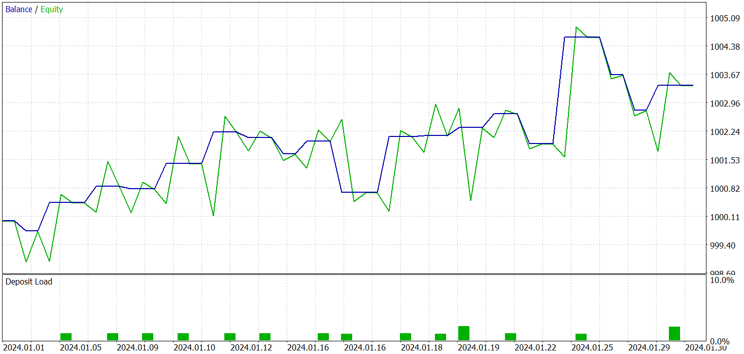
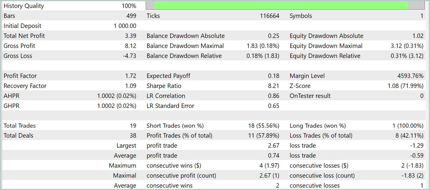
As a result of training, we obtained a policy capable of generating profit outside the training dataset. During the testing period, the model executed 19 trades, 11 of which were profitable (57.89%). By comparison, our previously implemented R-MAT model executed 15 trades over the same period, with 9 profitable trades (60.0%). Notably, the total return of the new model was nearly double that of the baseline.
Conclusion
The SAMformer framework provides an effective solution to the key limitations of the Transformer architecture in the context of long-term forecasting for multivariate time series. A conventional Transformer faces significant challenges, including high training complexity and poor generalization capability, particularly when working with small training datasets.
The core strengths of SAMformer lie in its shallow architecture and the integration of Sharpness-Aware Minimization (SAM). These approaches help the model avoid poor local minima, improve training stability and accuracy, and deliver superior generalization performance.
In the practical portion of our work, we implemented our own interpretation of these methods in MQL5 and trained the models on real historical data. The testing results validate the effectiveness of the proposed approaches, showing that their integration can enhance the performance of baseline models without incurring additional training costs. And in some cases, it even allows you to reduce such training costs.
References
Programs used in the article
| # | Name | Type | Description |
|---|---|---|---|
| 1 | Research.mq5 | Expert Advisor | Expert Advisor for collecting examples |
| 2 | ResearchRealORL.mq5 | Expert Advisor | Expert Advisor for collecting examples using the Real-ORL method |
| 3 | Study.mq5 | Expert Advisor | Model training Expert Advisor |
| 4 | StudyEncoder.mq5 | Expert Advisor | Encoder training Expert Advisor |
| 5 | Test.mq5 | Expert Advisor | Model testing Expert Advisor |
| 6 | Trajectory.mqh | Class library | System state description structure |
| 7 | NeuroNet.mqh | Class library | A library of classes for creating a neural network |
| 8 | NeuroNet.cl | Library | OpenCL program code library |
Translated from Russian by MetaQuotes Ltd.
Original article: https://www.mql5.com/ru/articles/16403
Warning: All rights to these materials are reserved by MetaQuotes Ltd. Copying or reprinting of these materials in whole or in part is prohibited.
This article was written by a user of the site and reflects their personal views. MetaQuotes Ltd is not responsible for the accuracy of the information presented, nor for any consequences resulting from the use of the solutions, strategies or recommendations described.

- Free trading apps
- Over 8,000 signals for copying
- Economic news for exploring financial markets
You agree to website policy and terms of use
Annual income of Russian banks in dolars. Divide by 12 and compare.
In yuan 6, in yuan bonds more than 10.
In renminbi 6, in renminbi bonds more than 10.
But the results of testing on EURUSD and the result in USD are given in the article. At the same time, the load on the deposit is 1-2%. And nobody wrote that it is a grail.
But the article gives the results of testing on EURUSD and the result in USD. At the same time, the load on the deposit is 1-2%. And no one wrote that it is a grail.
ok. cap in quid in banks give 5%.
Total profit of 0.35% per month? Wouldn't it be more profitable to just put the money in the bank?